sf / stars / sftime

NOTE:  This page has been revised for the 2024 version of the course, but there may be some additional edits.  

1 Introduction

In addition to the terra package, there are three other packages that are able to manage and analyze explicitly spatial and spatiotemporal data in R. These include

• sf (“simple features”) – the replacement for the original spatial sp package in R, that links directly with the GEOS, GDAL, and PROJ libraies, and thus enables a broad range of mapping (including projection and coordinate transformations), and the application of geospatial analyses to spatial data [https://r-spatial.github.io/sf/index.html];
• stars – an extension to sf, which explicity handles space-time data on regular grids (data cubes) (and is a replacement for the older spacetime package) [https://r-spatial.github.io/stars/index.html]; and
• sftime also an extension to the sf package, which explicity includes a “time” variable [https://r-spatial.org/r/2022/04/12/sftime-1.html].

Each of these packages has a typical application: for sf, general mapping and geospatial analyses, for stars, the analysis of data cubes like those generated by climate models, and for sftime, the analysis of data that are not necessarily on regular grids in time or space, like earthquake or paleoecological data. This is a really short introduction, the main reference is Pebesma, E. and R. Bivand, 2023, Spatial Data Science with Applications in R (CRC Press) [https://r-spatial.org/book/].

The sf package supports well the reading and writing of “traditional” geospatial data formats, such as ESRI Shapefiles, which is demonstrated here by reading a shape file from the NaturalEarth collection [https://www.naturalearthdata.com]. Load the libraries:

library(sf)
library(stars)
library(sftime)
library(terra)
library(tidyverse)
library(ggplot2)
library(RColorBrewer)

# load data from a saved .RData file
con <- url("https://pages.uoregon.edu/bartlein/RESS/RData/geog490.RData")
load(file=con) 

Read a previously downloaded shape file:

# world_sf
shapefile <- 
  "/Users/bartlein/Dropbox/DataVis/working/data/shp_files/ne_110m_admin_0_countries/ne_110m_admin_0_countries.shp"
world_sf <- st_read(shapefile)

## Reading layer `ne_110m_admin_0_countries' from data source 
##   `/Users/bartlein/Dropbox/DataVis/working/data/shp_files/ne_110m_admin_0_countries/ne_110m_admin_0_countries.shp' 
##   using driver `ESRI Shapefile'
## Simple feature collection with 177 features and 94 fields
## Geometry type: MULTIPOLYGON
## Dimension:     XY
## Bounding box:  xmin: -180 ymin: -90 xmax: 180 ymax: 83.64513
## Geodetic CRS:  WGS 84

Get the outline and plot it, and note the class of the world_otl_sf object

# get the just the outline (i.e. the st_geometry)
world_otl_sf <- st_geometry(world_sf)
plot(world_otl_sf) 

class(world_otl_sf)

## [1] "sfc_MULTIPOLYGON" "sfc"

Here’s a ggplot2() version of the world outline:

# ggplot map of world_outline
ggplot() + 
  geom_sf(data = world_otl_sf, fill = NA, col = "black") + 
  scale_x_continuous(breaks = seq(-180, 180, 30)) +
  scale_y_continuous(breaks = seq(-90, 90, 30)) +
  coord_sf(xlim = c(-180, +180), ylim = c(-90, 90), expand = FALSE) +
  theme_bw()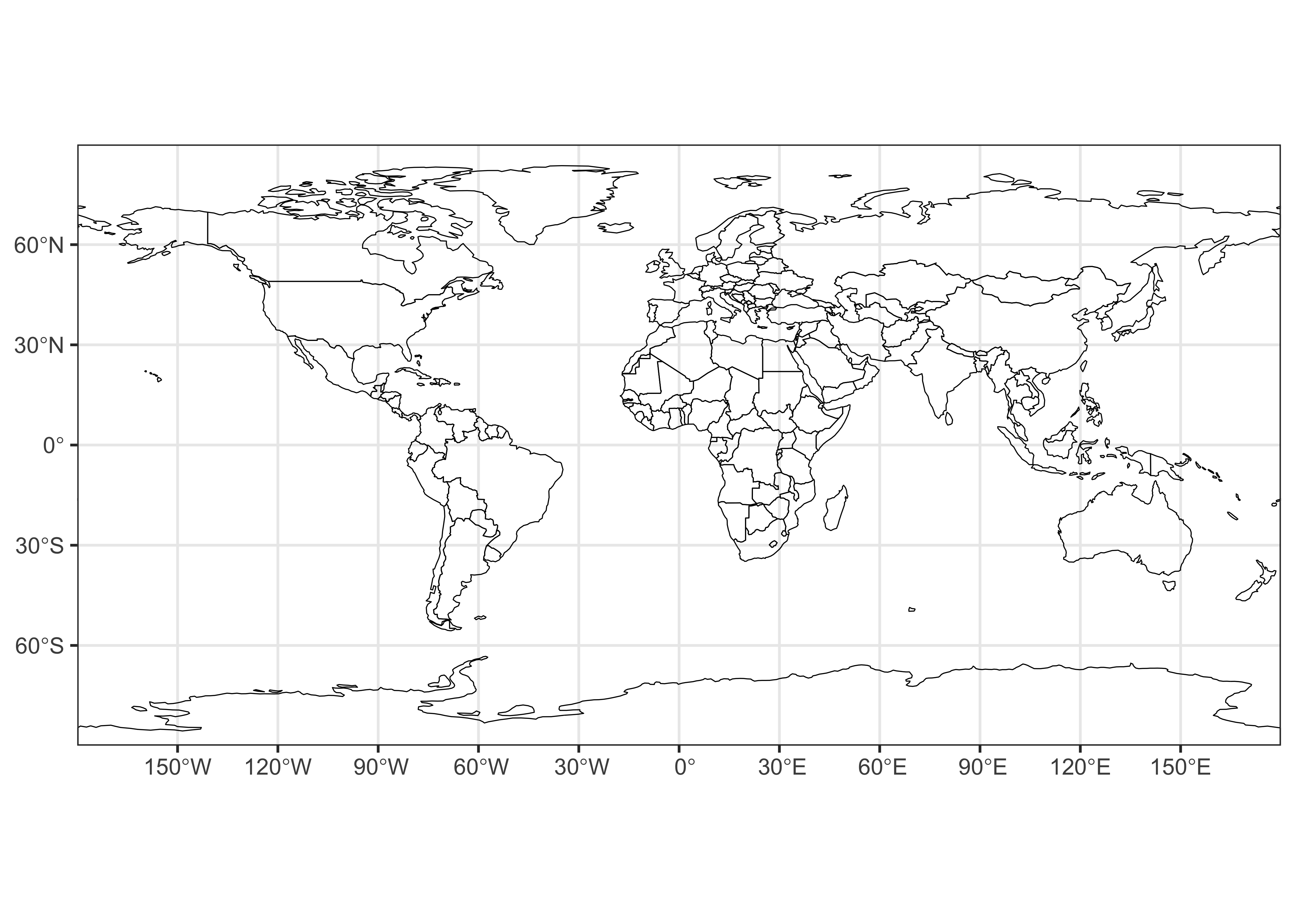

ggplot2 allows fine control of such things as graticule labeling, color scales, and so on.

2 stars

The stars package, like terra and sf can easily read and write netCDF files. Here, we’ll look at a couple of “reanalysis” datasets consisting of 4-dimensional cubes of retrospective long-term means of climate data generated by observations and a reanalysis climate model, where the dimensions are longitude by latitude by level by time (and level refers to elevation in the atmosphere as represented by pressure, e.g. level 1 is at1000 hPa (i.e., the surface), level 6 is at 500 hPa (upper air)).

2.1 Read some data

Read the pressure-surface heights:

# stars
nc_file <- "/Users/bartlein/Projects/RESS/data/nc_files/NCEP2_hgt.mon.ltm.1991-2020.nc"
hgt <- read_ncdf(nc_file, var = "hgt", proxy = FALSE)

# list some info
hgt

## stars object with 4 dimensions and 1 attribute
## attribute(s), summary of first 1e+05 cells:
##              Min.  1st Qu. Median     Mean  3rd Qu.    Max.
## hgt [m] -133.7667 1339.558 4405.3 5014.268 8540.267 12480.2
## dimension(s):
##       from  to offset delta  refsys                    values x/y
## lon      1 143 -181.2   2.5  WGS 84                      NULL [x]
## lat      1  73  91.25  -2.5  WGS 84                      NULL [y]
## level    1  17     NA    NA      NA          [17] 10,...,1000    
## time     1  12     NA    NA POSIXct 0000-12-30,...,0001-11-29

dim(hgt)

##   lon   lat level  time 
##   143    73    17    12

The time-dimension values in this data set are in the “time-since” format, which read_ncdf() interprets in a somewhat awkward year-month-day format. They can be replaced by text labels:

# replace time dimension values
attr(hgt, "dimensions")$time$values <- 
  c("Jan", "Feb", "Mar", "Apr", "May", "Jun", "Jul", "Aug", "Sep", "Oct", "Nov", "Dec")
attr(hgt, "dimensions")$time$refsys <- "Name"
hgt

## stars object with 4 dimensions and 1 attribute
## attribute(s), summary of first 1e+05 cells:
##              Min.  1st Qu. Median     Mean  3rd Qu.    Max.
## hgt [m] -133.7667 1339.558 4405.3 5014.268 8540.267 12480.2
## dimension(s):
##       from  to offset delta refsys           values x/y
## lon      1 143 -181.2   2.5 WGS 84             NULL [x]
## lat      1  73  91.25  -2.5 WGS 84             NULL [y]
## level    1  17     NA    NA     NA [17] 10,...,1000    
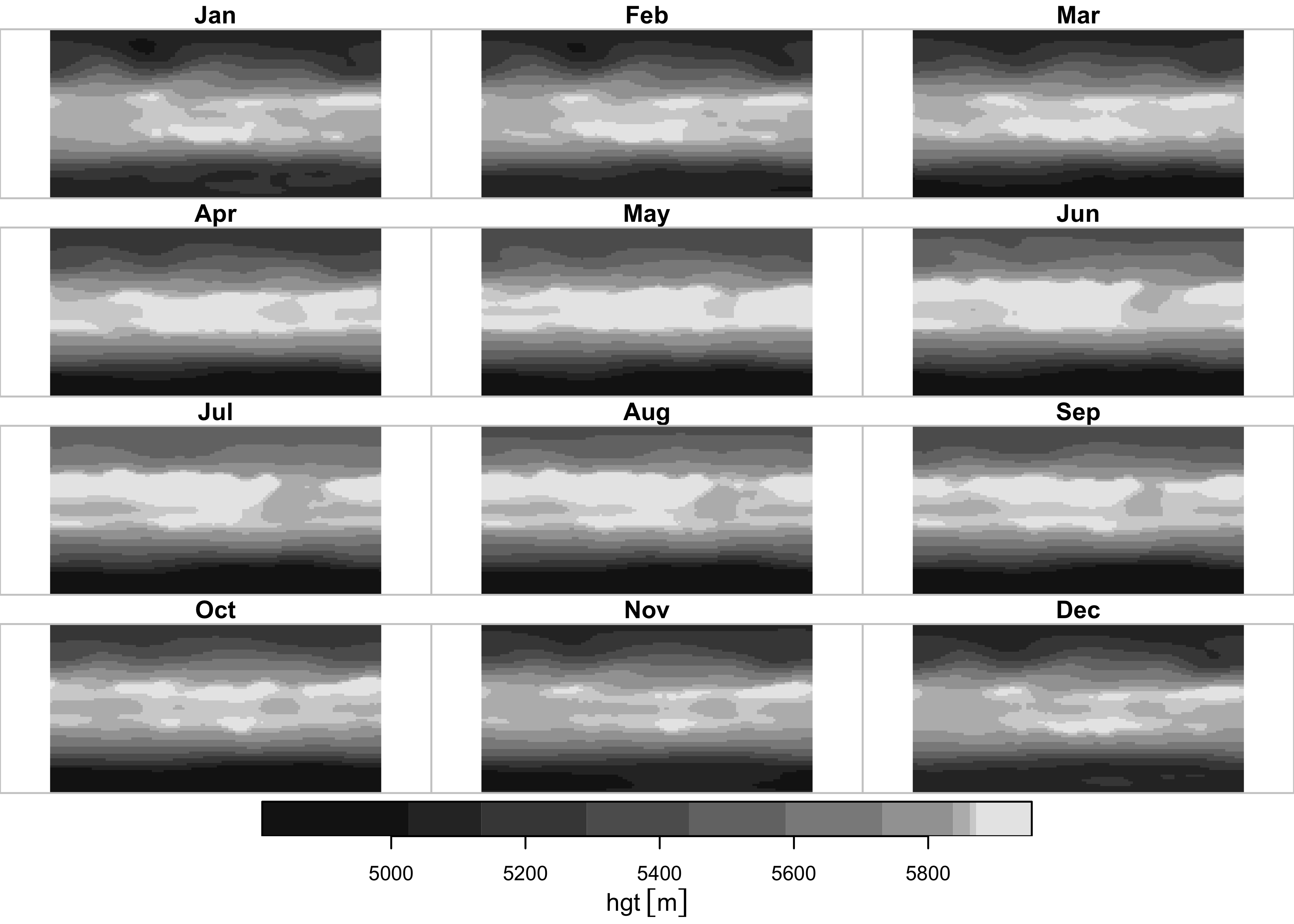
## time     1  12     NA    NA   Name      Jan,...,Dec

Plot the pressure-surface heights. Ignore the bounding-box warning.

plot(hgt)

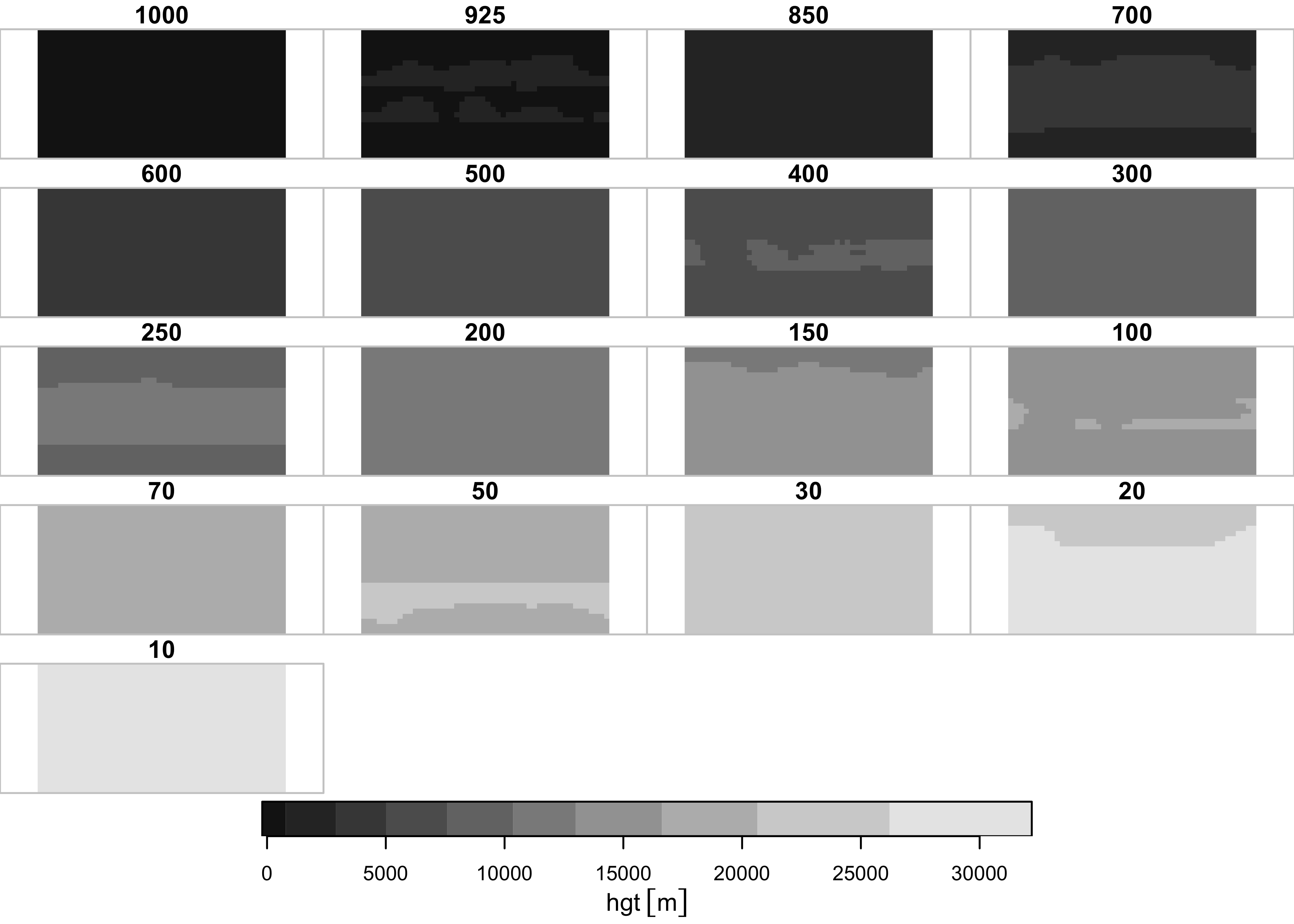
What seems to get plotted is the long-term means of one month at the different levels. Plot a single level, here level 6, or the 500 hPa level.

plot(slice(hgt, level,  6)) # level = 6 is 500 hPa

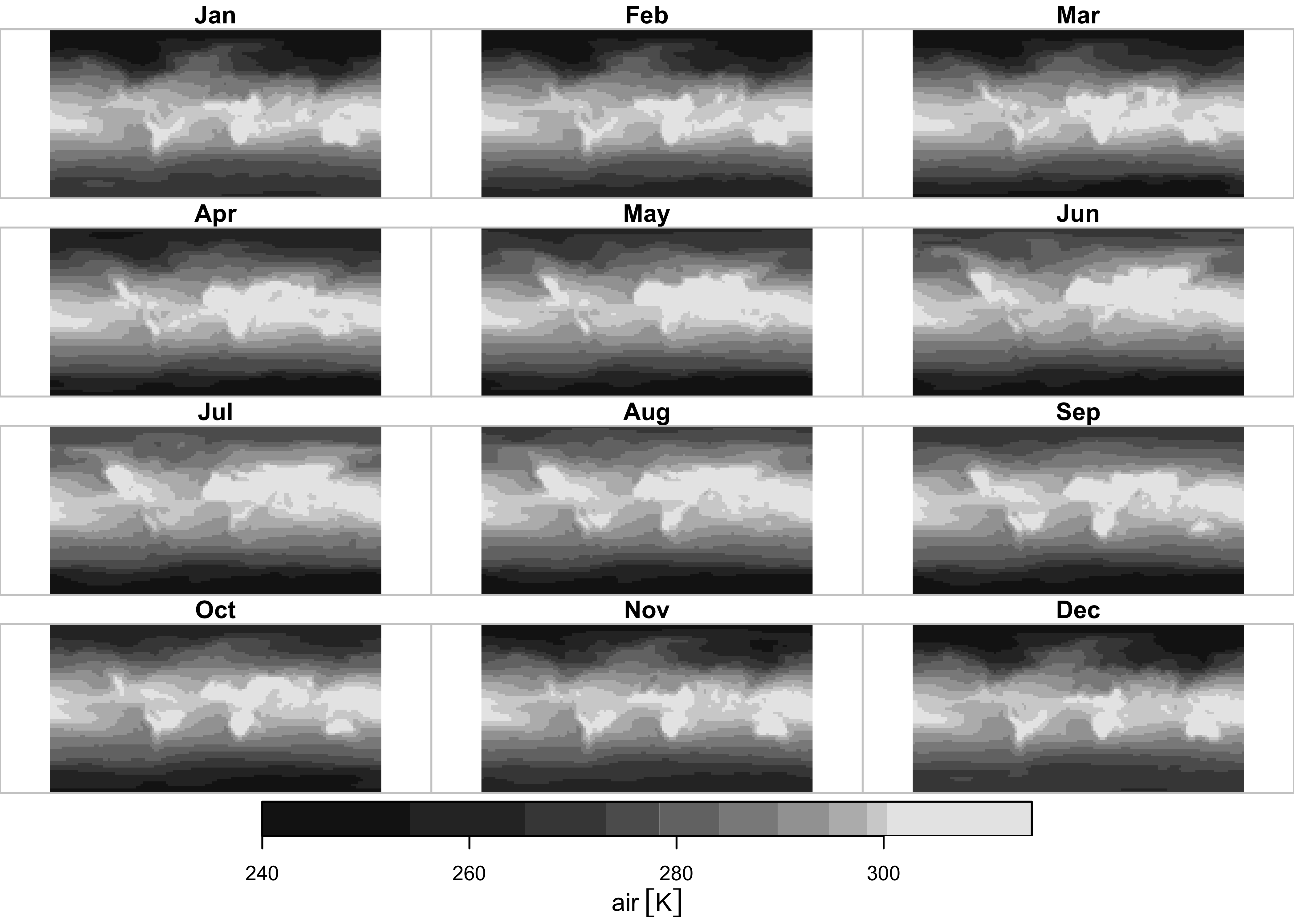
Repeat for air temperature (air in this data set):

nc_file <- "/Users/bartlein/Projects/RESS/data/nc_files/NCEP2_air.mon.ltm.1991-2020.nc"
air <- read_ncdf(nc_file, var = "air", proxy = FALSE)
air

## stars object with 4 dimensions and 1 attribute
## attribute(s), summary of first 1e+05 cells:
##            Min. 1st Qu.   Median    Mean  3rd Qu.     Max.
## air [K] 209.071 232.305 253.0591 253.473 273.3577 308.6734
## dimension(s):
##       from  to offset delta  refsys                    values x/y
## lon      1 143 -181.2   2.5  WGS 84                      NULL [x]
## lat      1  73  91.25  -2.5  WGS 84                      NULL [y]
## level    1  17     NA    NA      NA          [17] 10,...,1000    
## time     1  12     NA    NA POSIXct 0000-12-30,...,0001-11-29

dim(air)

##   lon   lat level  time 
##   143    73    17    12

# replace time dimension values
attr(air, "dimensions")$time$values <- 
  c("Jan", "Feb", "Mar", "Apr", "May", "Jun", "Jul", "Aug", "Sep", "Oct", "Nov", "Dec")
attr(air, "dimensions")$time$refsys <- "Name"
air

## stars object with 4 dimensions and 1 attribute
## attribute(s), summary of first 1e+05 cells:
##            Min. 1st Qu.   Median    Mean  3rd Qu.     Max.
## air [K] 209.071 232.305 253.0591 253.473 273.3577 308.6734
## dimension(s):
##       from  to offset delta refsys           values x/y
## lon      1 143 -181.2   2.5 WGS 84             NULL [x]
## lat      1  73  91.25  -2.5 WGS 84             NULL [y]
## level    1  17     NA    NA     NA [17] 10,...,1000    
## time     1  12     NA    NA   Name      Jan,...,Dec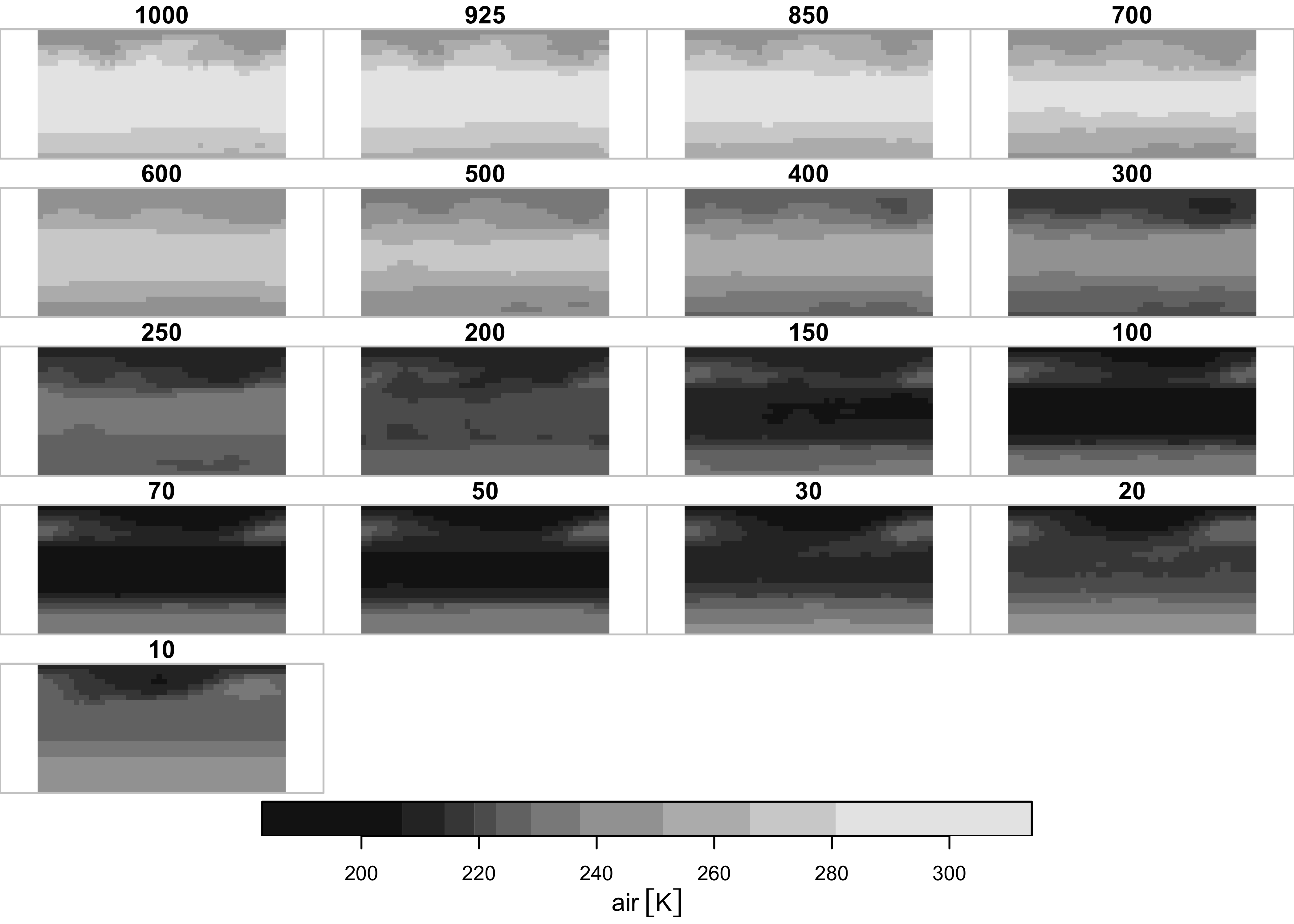

plot(air)

plot(slice(air, level,  1)) # level 1 is 1000 hPa (surface)

2.2 ggplot2 maps

ggplot2 has a function geom_stars() that “knows” how to plot stars data objects: Here’s a plot of 500 hPa (level 6) heights:

# stars ggplots
ggplot() +
  geom_stars(data = slice(hgt, level, 6)) +
  geom_sf(data = world_otl_sf, fill = NA) +
  facet_wrap(~ time, nrow = 4, ncol = 3) +
  coord_sf(xlim = c(-180, +180), ylim = c(-90, 90), expand = FALSE) +
  scale_fill_distiller(palette = "PuOr") +
  theme_bw() + theme(strip.text = element_text(size = 6))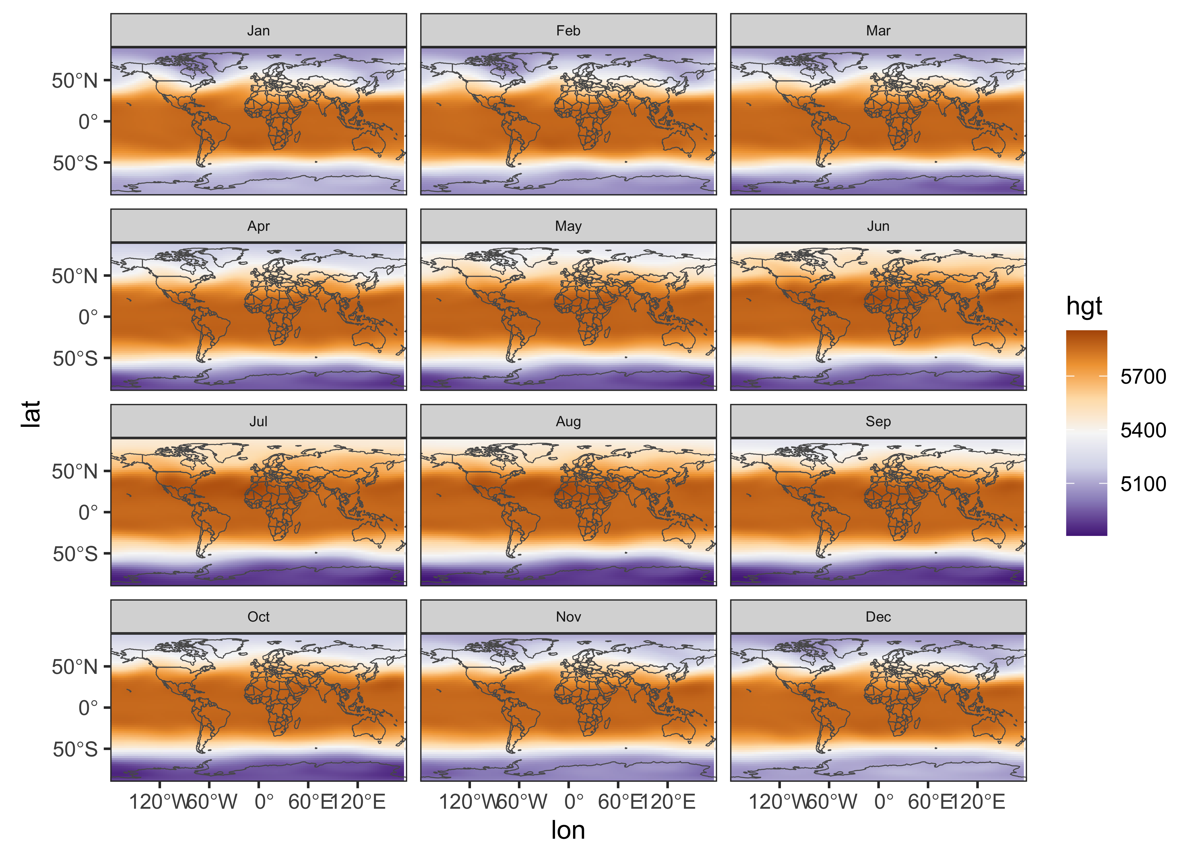

Here, the stars object was plotted first, followed by the world world outline. The facet_wrap() function controls the paneling, and the expand = FALSE argument of the coord_sf() function removes some of the white space between panels. The theme(strip.text = element_text(size = 6)) function makes the “header” boxes and fonts a little smaller.

Here’s the plot for near-surface air temperature:

ggplot() +
  geom_stars(data = slice(air, level, 1)) + 
  geom_sf(data = world_otl_sf, fill = NA) +
  facet_wrap(~ time, nrow = 4, ncol = 3) +
  coord_sf(xlim = c(-180, +180), ylim = c(-90, 90), expand = FALSE) +
  scale_fill_distiller(palette = "RdBu") +
  theme_bw() + theme(strip.text = element_text(size = 6))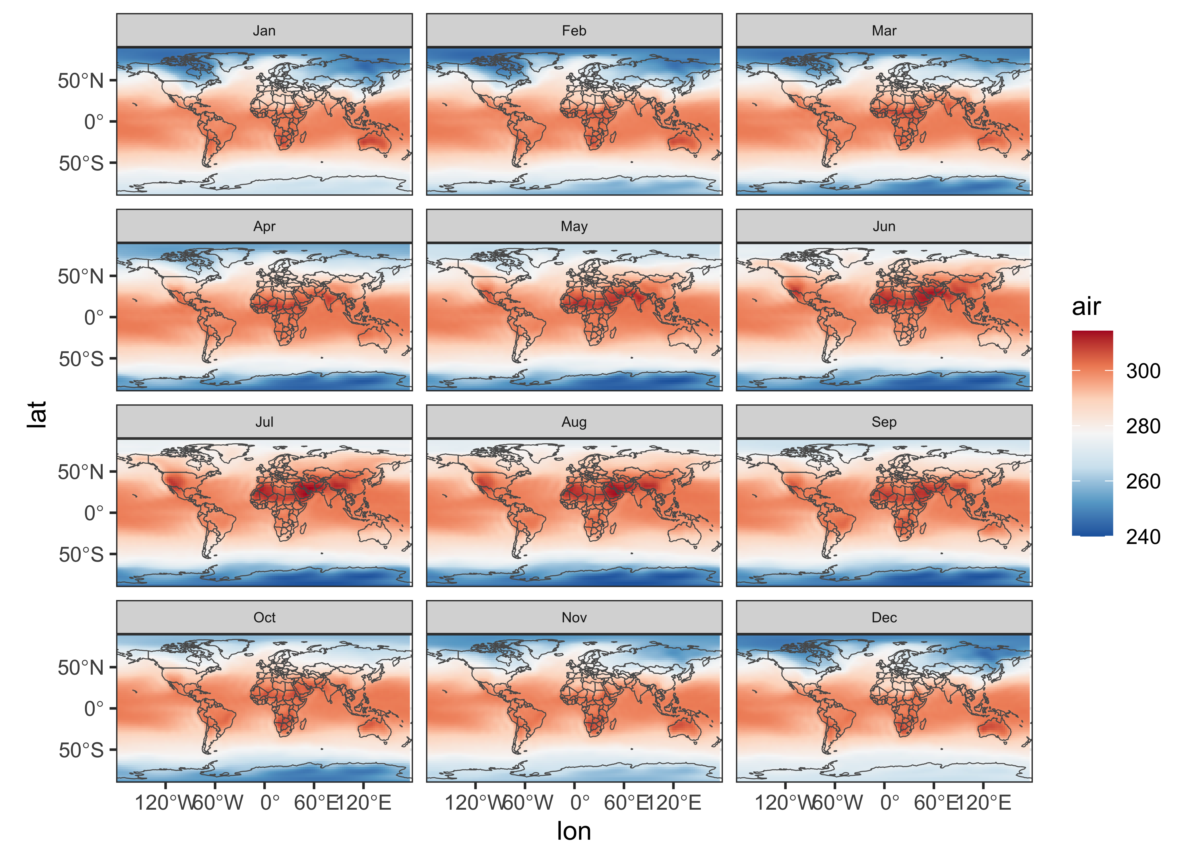

2.3 Converting stars objects to terra and sf objects

stars objects, in particular 3-dimensional data cubes, can be easily converted to terra and sf objects (i.e. raster stacks, or SpatRaster objects in terra and in sf). To demonstrate this, get a single 3-d “slice” of air temperature from the 4-d cube:

# get a single slice
class(air)

## [1] "stars"

dim(air)

##   lon   lat level  time 
##   143    73    17    12

So air is a 4-d object. Now get the slice (at 1000 hPa):

air_1000 <- slice(air, level,  1)
class(air_1000)

## [1] "stars"

air_1000

## stars object with 3 dimensions and 1 attribute
## attribute(s):
##             Min.  1st Qu.   Median     Mean 3rd Qu.    Max.
## air [K] 239.9924 269.3894 284.1218 281.2621  296.84 314.302
## dimension(s):
##      from  to offset delta refsys      values x/y
## lon     1 143 -181.2   2.5 WGS 84        NULL [x]
## lat     1  73  91.25  -2.5 WGS 84        NULL [y]
## time    1  12     NA    NA   Name Jan,...,Dec

dim(air_1000)

##  lon  lat time 
##  143   73   12

Now convert that 3-d slice to terra

# convert to SpatRaster
air_1000_sr <- as(air_1000, "SpatRaster") 
class(air_1000_sr)

## [1] "SpatRaster"
## attr(,"package")
## [1] "terra"

air_1000_sr

## class       : SpatRaster 
## dimensions  : 73, 143, 12  (nrow, ncol, nlyr)
## resolution  : 2.5, 2.5  (x, y)
## extent      : -181.25, 176.25, -91.25, 91.25  (xmin, xmax, ymin, ymax)
## coord. ref. : lon/lat WGS 84 
## source(s)   : memory
## names       :      Jan,      Feb,      Mar,      Apr,      May,      Jun, ... 
## min values  : 244.2550, 244.2596, 245.4530, 241.4906, 239.9924, 240.1938, ... 
## max values  : 308.6734, 307.2127, 307.9087, 309.1877, 311.3960, 313.2636, ...

Notice that the spatial extent is a little odd. We know from the original netCDF file that the western edge of the grid is at -180.0E, and the southern edge at -90.0N. The correct spatial exent can be restored like this:

# restore spatial extent
ext(air_1000_sr) <- c(-180, 175, -90, 90)

The dataset, which is now a terra object, can be plotted as usual:

panel(air_1000_sr, nc = 3, nr = 4)

Similarly, the stars object, air_1000, can be converted to an sf object:

# convert stars to sf
air_1000_sf <- st_as_sf(air_1000, as_points = TRUE)
air_1000_sf

## Simple feature collection with 10439 features and 12 fields
## Geometry type: POINT
## Dimension:     XY
## Bounding box:  xmin: -180 ymin: -90 xmax: 175 ymax: 90
## Geodetic CRS:  WGS 84
## First 10 features:
##            Jan          Feb         Mar          Apr          May          Jun          Jul          Aug
## 1  248.043 [K] 247.7463 [K] 248.732 [K] 255.4446 [K] 265.0327 [K] 272.6674 [K] 274.6298 [K] 272.8947 [K]
## 2  248.043 [K] 247.7463 [K] 248.732 [K] 255.4446 [K] 265.0327 [K] 272.6674 [K] 274.6298 [K] 272.8947 [K]
## 3  248.043 [K] 247.7463 [K] 248.732 [K] 255.4446 [K] 265.0327 [K] 272.6674 [K] 274.6298 [K] 272.8947 [K]
## 4  248.043 [K] 247.7463 [K] 248.732 [K] 255.4446 [K] 265.0327 [K] 272.6674 [K] 274.6298 [K] 272.8947 [K]
## 5  248.043 [K] 247.7463 [K] 248.732 [K] 255.4446 [K] 265.0327 [K] 272.6674 [K] 274.6298 [K] 272.8947 [K]
## 6  248.043 [K] 247.7463 [K] 248.732 [K] 255.4446 [K] 265.0327 [K] 272.6674 [K] 274.6298 [K] 272.8947 [K]
## 7  248.043 [K] 247.7463 [K] 248.732 [K] 255.4446 [K] 265.0327 [K] 272.6674 [K] 274.6298 [K] 272.8947 [K]
## 8  248.043 [K] 247.7463 [K] 248.732 [K] 255.4446 [K] 265.0327 [K] 272.6674 [K] 274.6298 [K] 272.8947 [K]
## 9  248.043 [K] 247.7463 [K] 248.732 [K] 255.4446 [K] 265.0327 [K] 272.6674 [K] 274.6298 [K] 272.8947 [K]
## 10 248.043 [K] 247.7463 [K] 248.732 [K] 255.4446 [K] 265.0327 [K] 272.6674 [K] 274.6298 [K] 272.8947 [K]
##             Sep          Oct          Nov          Dec          geometry
## 1  267.3551 [K] 259.2516 [K] 252.7007 [K] 249.3092 [K]   POINT (-180 90)
## 2  267.3551 [K] 259.2516 [K] 252.7007 [K] 249.3092 [K] POINT (-177.5 90)
## 3  267.3551 [K] 259.2516 [K] 252.7007 [K] 249.3092 [K]   POINT (-175 90)
## 4  267.3551 [K] 259.2516 [K] 252.7007 [K] 249.3092 [K] POINT (-172.5 90)
## 5  267.3551 [K] 259.2516 [K] 252.7007 [K] 249.3092 [K]   POINT (-170 90)
## 6  267.3551 [K] 259.2516 [K] 252.7007 [K] 249.3092 [K] POINT (-167.5 90)
## 7  267.3551 [K] 259.2516 [K] 252.7007 [K] 249.3092 [K]   POINT (-165 90)
## 8  267.3551 [K] 259.2516 [K] 252.7007 [K] 249.3092 [K] POINT (-162.5 90)
## 9  267.3551 [K] 259.2516 [K] 252.7007 [K] 249.3092 [K]   POINT (-160 90)
## 10 267.3551 [K] 259.2516 [K] 252.7007 [K] 249.3092 [K] POINT (-157.5 90)

class(air_1000_sf)

## [1] "sf"         "data.frame"

The argument as_points = TRUE indicates that we would like to convert to an sf POINT geometry type. Setting as_points = FALSE will yield, in this case, an sf geometry type of POLYGON, which would be less efficent for storing the data.

3 sf

Plot the sf object just created, first as a set of panels, one for each month, then as a single map for January:

plot(air_1000_sf, max.plot = 12)

plot(air_1000_sf[,1])

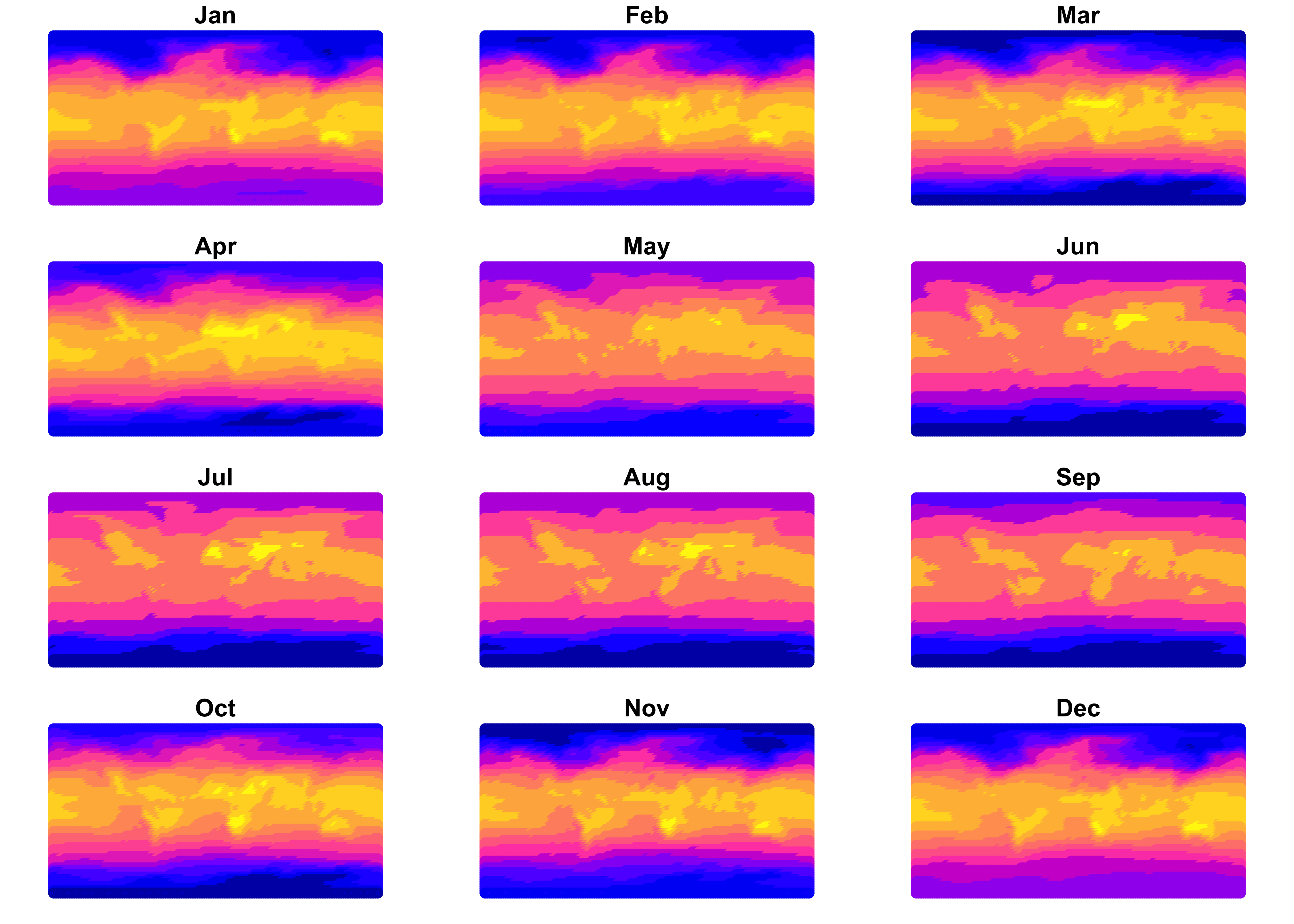
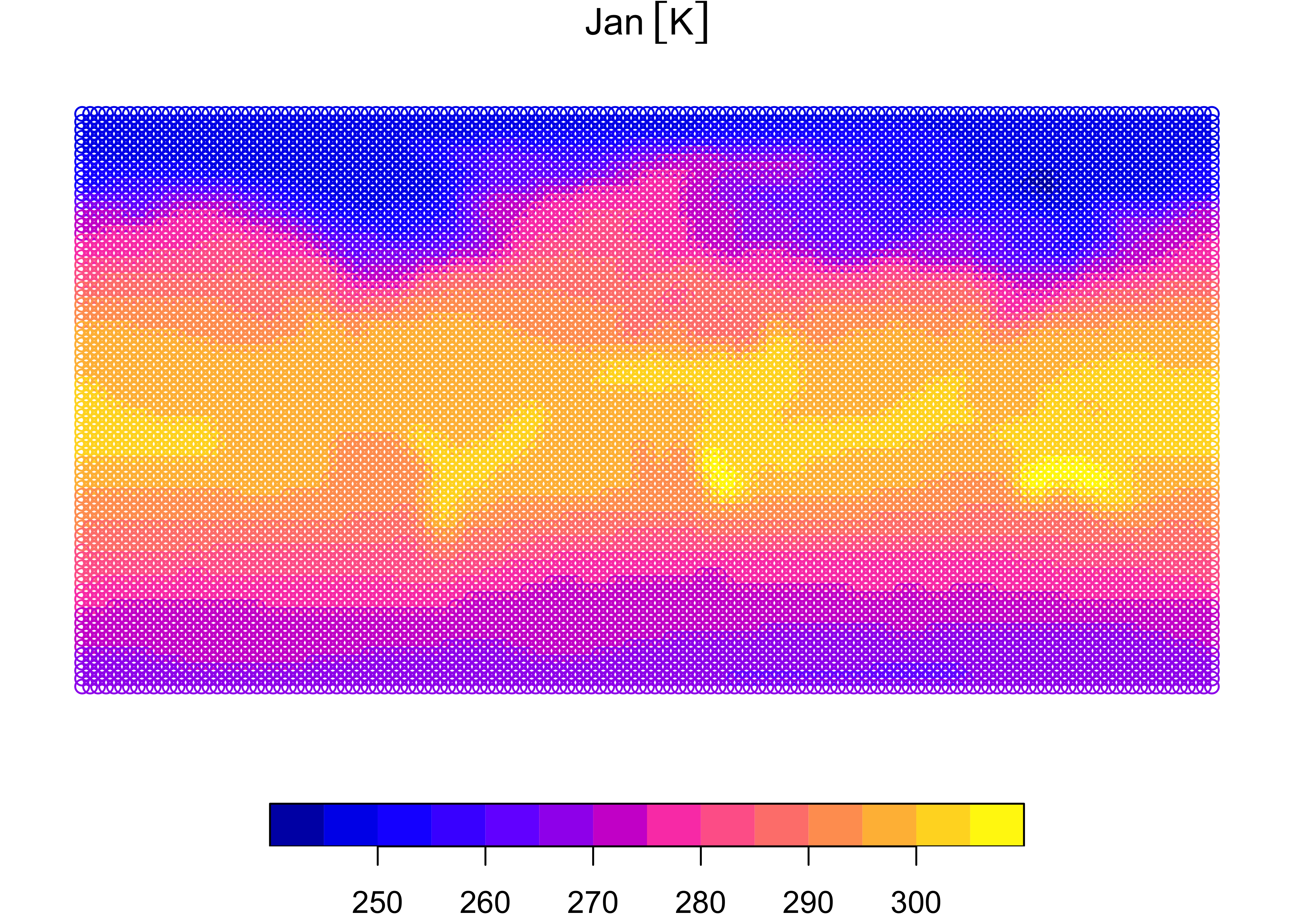
The January map clearly shows that the data consist of individual points.

3.1 ggplot2 maps

To produce ggplot2 maps of the air1000_sf object, there are several strategies. One is to first convert the raster brick here to a data.frame, which could subsequently analyzed. Extract the coordinates and data, in this case for January, from the air1000_sf object:

# make a data.frame
lon <- st_coordinates(air_1000_sf)[,1]
lat <- st_coordinates(air_1000_sf)[,2]
air <- as.vector((air_1000_sf[,1]$Jan))
air_1000_df <- data.frame(lon, lat, air)
dim(air_1000_df)

## [1] 10439     3

A little more set-up. Create a set of axis labels:

# axis labels (breaks)
breaks_x <- c(seq(-180, 180, by = 60)) 
breaks_y <- c(seq(-90, 90, by = 30)) 
labels_x <- as.character(breaks_x) 
labels_y <- as.character(breaks_y) 

Make a graticule.

# make a graticule 
grat = st_graticule(air_1000_sf, lon = breaks_x, lat = breaks_y)
grat

## Simple feature collection with 10 features and 10 fields
## Geometry type: LINESTRING
## Dimension:     XY
## Bounding box:  xmin: -179.82 ymin: -89.91 xmax: 175 ymax: 89.91
## Geodetic CRS:  WGS 84
##    degree type   degree_label                       geometry x_start y_start x_end  y_end angle_start
## 2    -120    E "120"*degree*W LINESTRING (-120 -89.91, -1... -120.00  -89.91  -120  89.91          90
## 3     -60    E " 60"*degree*W LINESTRING (-60 -89.91, -60...  -60.00  -89.91   -60  89.91          90
## 4       0    E   "  0"*degree LINESTRING (0 -89.91, 0 -88...    0.00  -89.91     0  89.91          90
## 5      60    E " 60"*degree*E LINESTRING (60 -89.91, 60 -...   60.00  -89.91    60  89.91          90
## 6     120    E "120"*degree*E LINESTRING (120 -89.91, 120...  120.00  -89.91   120  89.91          90
## 8     -60    N  "60"*degree*S LINESTRING (-179.82 -60, -1... -179.82  -60.00   175 -60.00           0
## 9     -30    N  "30"*degree*S LINESTRING (-179.82 -30, -1... -179.82  -30.00   175 -30.00           0
## 10      0    N    " 0"*degree LINESTRING (-179.82 0, -176... -179.82    0.00   175   0.00           0
## 11     30    N  "30"*degree*N LINESTRING (-179.82 30, -17... -179.82   30.00   175  30.00           0
## 12     60    N  "60"*degree*N LINESTRING (-179.82 60, -17... -179.82   60.00   175  60.00           0
##    angle_end plot12
## 2         90   TRUE
## 3         90   TRUE
## 4         90   TRUE
## 5         90   TRUE
## 6         90   TRUE
## 8          0   TRUE
## 9          0   TRUE
## 10         0   TRUE
## 11         0   TRUE
## 12         0   TRUE

grat_otl <- st_geometry(grat)
plot(grat_otl)

Now a ggplot2 map:

# ggplot2 map of air
ggplot() +
  geom_tile(data = air_1000_df[,,1], aes(x = lon, y = lat, fill = air)) +
  scale_fill_gradient2(low = "darkblue", mid="white", high = "darkred", midpoint = 273.15) +
  geom_sf(data = world_otl_sf, col = "black", fill = NA) +
  geom_sf(data = grat_otl, col = "gray80", lwd = 0.5, lty = 3) +
  coord_sf(xlim = c(-180, +175.0), ylim = c(-90, 90), expand = FALSE) +
  scale_x_continuous(breaks = breaks_x) +
  scale_y_continuous(breaks = breaks_y) +
  labs(x = "Longitude", y = "Latitude", title="NCEP2 Reanalysis 2m Air Temperature", fill="K") +
  theme_bw()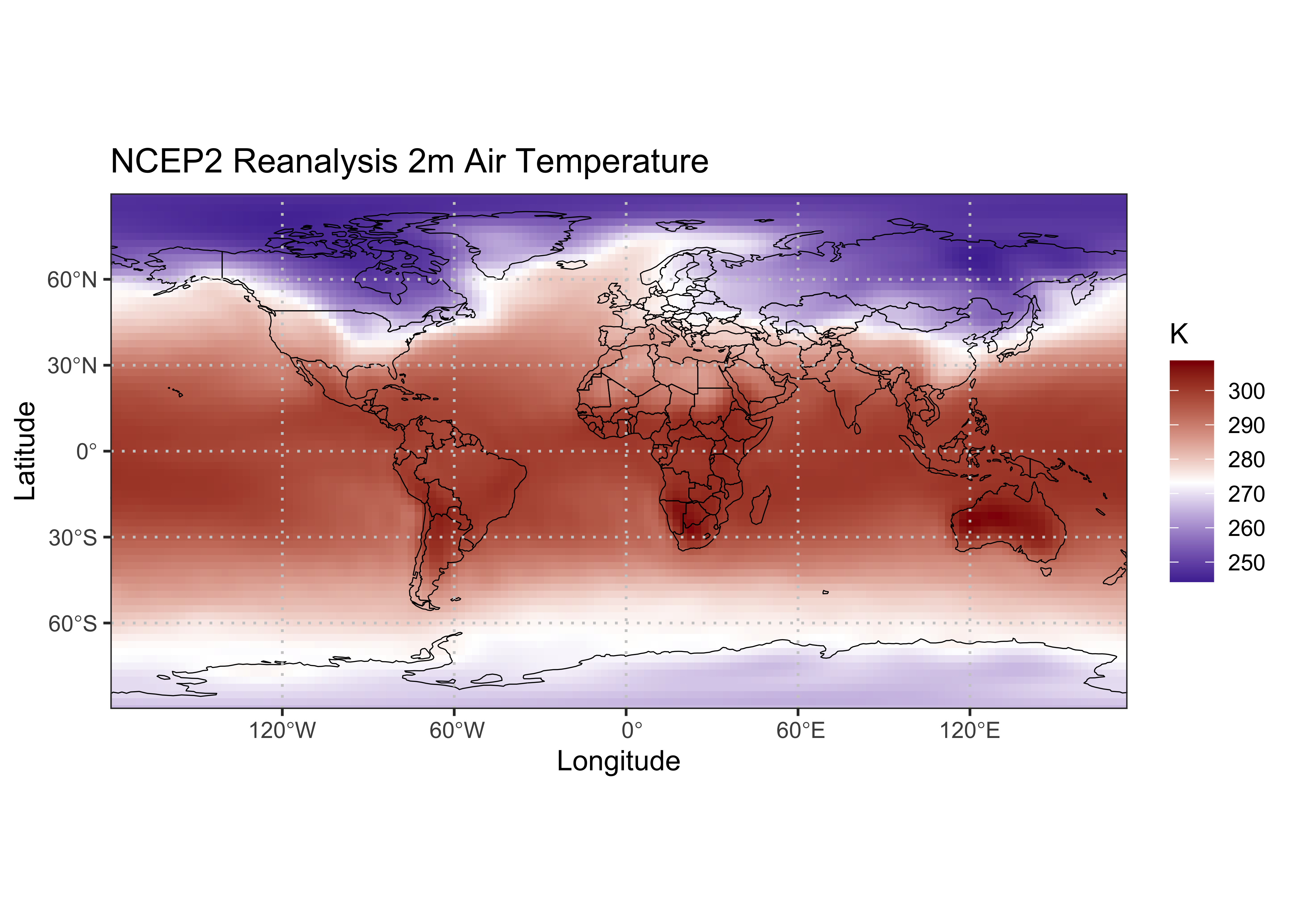

The geom_tile() function is an alternative to geom_point(), which fills in the spaces between points (plotting the data a tiles as opposed to round symbols). The two geom_sf() functions plot the world outline and graticule, and the coord_sf() function sets the ranges of the axes.

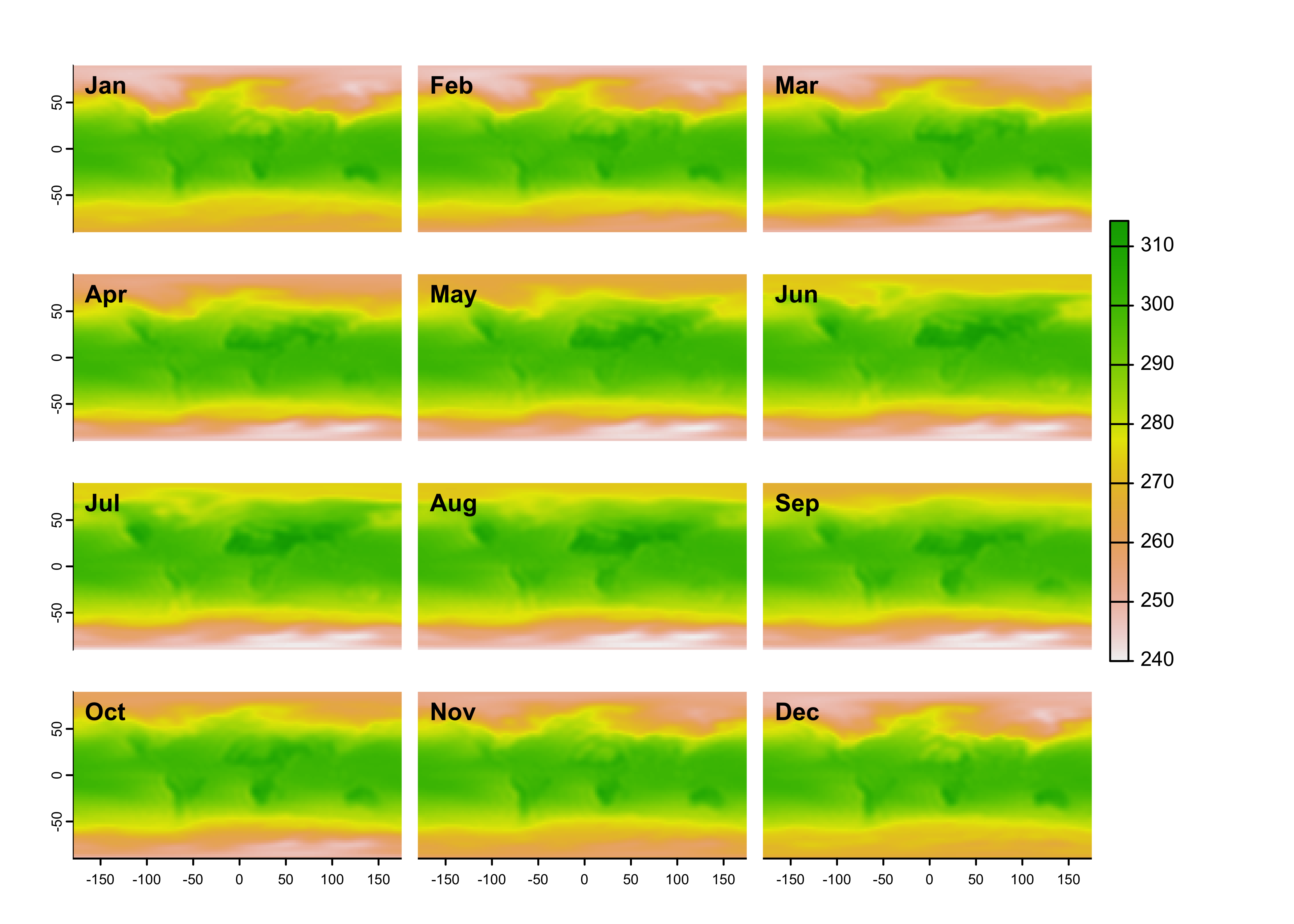
To make a multipanel map, create a second, long, data.frame, stacking the individual blocks of data for each month, and adding a month-name column. Begin by coverting the air_1000_sr SpatRaster object to a plain array:

# convert SpatRaster to a plain array
air_1000_sr

## class       : SpatRaster 
## dimensions  : 73, 143, 12  (nrow, ncol, nlyr)
## resolution  : 2.482517, 2.465753  (x, y)
## extent      : -180, 175, -90, 90  (xmin, xmax, ymin, ymax)
## coord. ref. : lon/lat WGS 84 
## source(s)   : memory
## names       :      Jan,      Feb,      Mar,      Apr,      May,      Jun, ... 
## min values  : 244.2550, 244.2596, 245.4530, 241.4906, 239.9924, 240.1938, ... 
## max values  : 308.6734, 307.2127, 307.9087, 309.1877, 311.3960, 313.2636, ...

dim(air_1000_sr)

## [1]  73 143  12

air_array <- as.array(air_1000_sr)
class(air_array)

## [1] "array"

dim(air_array)

## [1]  73 143  12

# unwrap the array to a long vector, stacking the months
air_1000_vector <- as.vector(air_array)
class(air_1000_vector)

## [1] "numeric"

length(air_1000_vector)

## [1] 125268

head(air_1000_vector)

## [1] 248.0430 247.4417 247.3460 247.8183 248.3500 248.9583

tail(air_1000_vector)

## [1] 269.5500 269.0778 269.3746 269.1017 267.7076 266.3626

Get the total lenght of one month’s worth of data in the stacked vector:

nt <- dim(air_array)[1] * dim(air_array)[2]
nt

## [1] 10439

Generate a new set of lons and lats for stacked vector:

# generate a "long" vector of lons and lats
lon2 <- seq(-180.0, 175.0, by = 2.5)
lat2 <- seq( 90.0,  -90.0, by = -2.5) # reverse the order
length(lon2); length(lat2)

## [1] 143

## [1] 73

lonlat <- (as.matrix(expand.grid(lat2, lon2)))
dim(lonlat)

## [1] 10439     2

Generate the month-names

# month names
month <- c(rep("Jan", nt), rep("Feb", nt), rep("Mar", nt), rep("Apr", nt), rep("May", nt), rep("Jun", nt),
  rep("Jul", nt), rep("Aug", nt), rep("Sep", nt), rep("Oct", nt), rep("Nov", nt), rep("Dec", nt))
length(month)

## [1] 125268

head(month); tail(month)

## [1] "Jan" "Jan" "Jan" "Jan" "Jan" "Jan"

## [1] "Dec" "Dec" "Dec" "Dec" "Dec" "Dec"

Make the data.frame. Note that the length of month is shorter than the lengths of the other columns, but it is replicated when building the data.frame:

# make the second data.frame
air_1000_df2 <- data.frame(lonlat[,2], lonlat[,1], air_1000_vector, month)
head(air_1000_df2)

##   lonlat...2. lonlat...1. air_1000_vector month
## 1        -180        90.0        248.0430   Jan
## 2        -180        87.5        247.4417   Jan
## 3        -180        85.0        247.3460   Jan
## 4        -180        82.5        247.8183   Jan
## 5        -180        80.0        248.3500   Jan
## 6        -180        77.5        248.9583   Jan

tail(air_1000_df2)

##        lonlat...2. lonlat...1. air_1000_vector month
## 125263         175       -77.5        269.5500   Dec
## 125264         175       -80.0        269.0778   Dec
## 125265         175       -82.5        269.3746   Dec
## 125266         175       -85.0        269.1017   Dec
## 125267         175       -87.5        267.7076   Dec
## 125268         175       -90.0        266.3626   Dec

names(air_1000_df2) <- c("lon", "lat", "air", "month")
dim(air_1000_df2)

## [1] 125268      4

Make the map:

# ggplot2 map of air
ggplot() + 
  geom_tile(data = air_1000_df2, aes(x = lon, y = lat, fill = air)) +
  geom_sf(data = world_otl_sf, col = "black", fill = NA) +
  geom_sf(data = grat_otl, col = "gray80", lwd = 0.5, lty = 3) +
  coord_sf(xlim = c(-180, +175), ylim = c(-90, 90), expand = FALSE) +
  facet_wrap(~factor(month, levels = 
    c("Jan", "Feb", "Mar", "Apr", "May", "Jun", "Jul", "Aug", "Sep", "Oct", "Nov", "Dec")), nrow = 4, ncol = 3) +
  scale_fill_gradient2(low = "darkblue", mid="white", high = "darkred", midpoint = 273.15) +
  # scale_y_continuous(breaks = seq(-90, 90, 90), expand = c(0,0)) +  # removes whitespace within panels
  # scale_x_continuous(breaks = seq(-180, 180, 90), expand = c(0,0)) +
  scale_x_continuous(breaks = breaks_x) +
  scale_y_continuous(breaks = breaks_y) +
  labs(title="NCEP2 Reanalysis 2m Air Temperature", fill="K") + 
  theme_bw() + theme(strip.text = element_text(size = 5))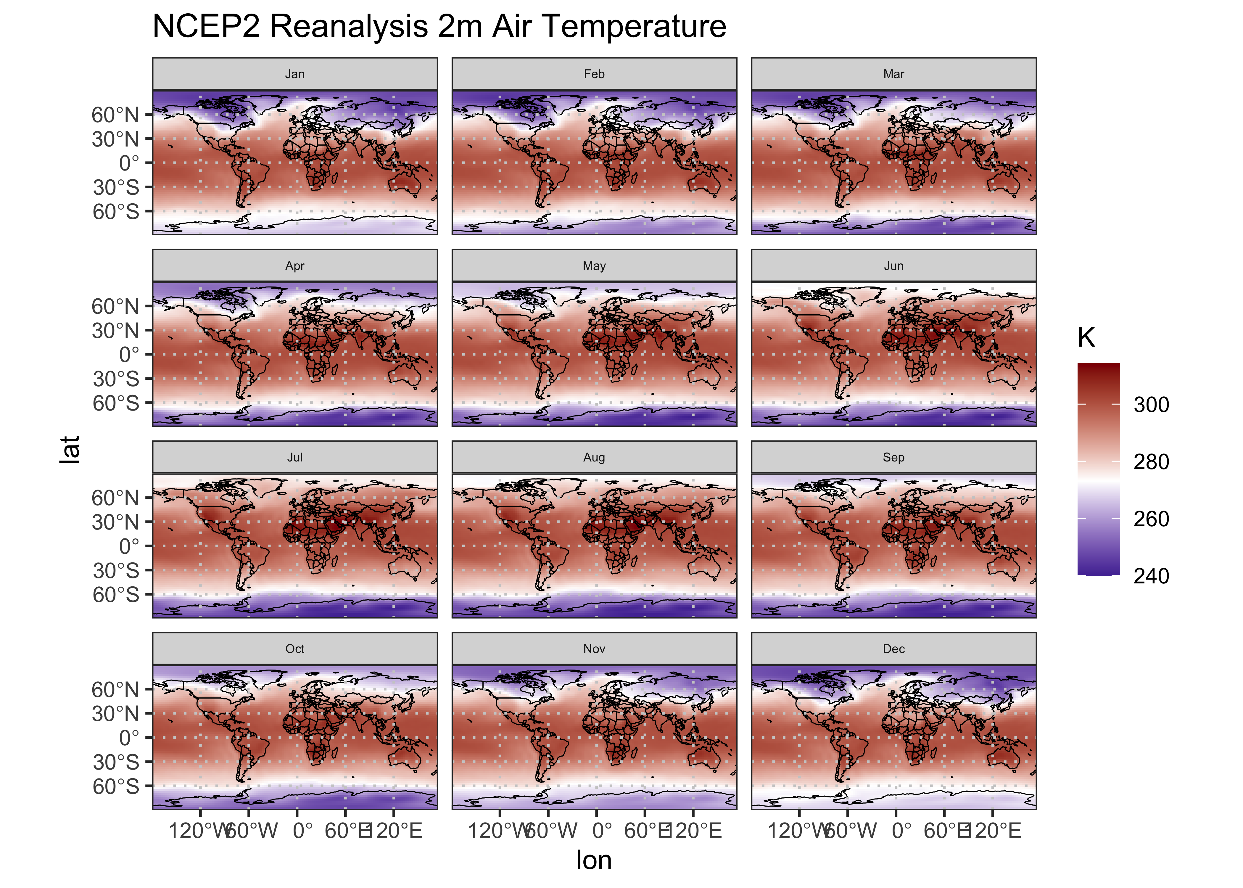

4 sftime

The sftime package is an extension of st to accomodate a time variable. Unlike stars the time are not expected to be regular, which can accomodate such data as earthquakes, fires, trajectories, etc. Here’s an example using a data set of paleo charcoal from the western U.S., used in Marlon et al. (2012) Long-term perspective on wildfires in the western USA. Proceedings of the National Academy of Sciences 109:E535-E543. [https://doi.org/10.1073/pnas.1112839109]. The data consist of z-scores of transformed charcoal-influx values (CHAR) for the past 3000 years, which record fire activity.

Read the data:

csv_path <- "/Users/bartlein/Dropbox/DataVis/working/data/csv_files/"
csv_file <- "wus_lat_trans.csv"
wus_char_csv <- read.csv((paste(csv_path, csv_file, sep = "")))
class(wus_char_csv)

## [1] "data.frame"

head(wus_char_csv)

##   seqnum sitenum  age ztinflux      lat       lon
## 1      1      39 -8.3   0.1150 33.65833 -117.8583
## 2      1      39 21.1  -0.2459 33.65833 -117.8583
## 3      1      39 41.2   2.5340 33.65833 -117.8583
## 4      1      39 50.7   1.8109 33.65833 -117.8583
## 5      1      39 68.8   1.8991 33.65833 -117.8583
## 6      1      39 88.0   1.0188 33.65833 -117.8583

Convert to a sftime object:

wus_char_sftime <- st_as_sftime(wus_char_csv, time_column_name = "age", coords = c("lon", "lat"),
        remove = FALSE, time_column_last = FALSE)
class(wus_char_sftime)

## [1] "sftime"     "sf"         "data.frame"

wus_char_sftime

## Spatiotemporal feature collection with 9999 features and 5 fields
## Geometry type: POINT
## Dimension:     XY
## Bounding box:  xmin: -124.8444 ymin: 33.65833 xmax: -105.5 ymax: 48.67222
## CRS:           NA
## Time column with classes: ''.
## Ranging from -74.6 to 3199.42.
## First 10 features:
##    seqnum sitenum   age ztinflux      lat       lon                   geometry
## 1       1      39  -8.3   0.1150 33.65833 -117.8583 POINT (-117.8583 33.65833)
## 2       1      39  21.1  -0.2459 33.65833 -117.8583 POINT (-117.8583 33.65833)
## 3       1      39  41.2   2.5340 33.65833 -117.8583 POINT (-117.8583 33.65833)
## 4       1      39  50.7   1.8109 33.65833 -117.8583 POINT (-117.8583 33.65833)
## 5       1      39  68.8   1.8991 33.65833 -117.8583 POINT (-117.8583 33.65833)
## 6       1      39  88.0   1.0188 33.65833 -117.8583 POINT (-117.8583 33.65833)
## 7       1      39 102.8   3.2354 33.65833 -117.8583 POINT (-117.8583 33.65833)
## 8       1      39 123.6   3.1590 33.65833 -117.8583 POINT (-117.8583 33.65833)
## 9       1      39 153.7   1.6399 33.65833 -117.8583 POINT (-117.8583 33.65833)
## 10      1      39 188.6   0.4108 33.65833 -117.8583 POINT (-117.8583 33.65833)

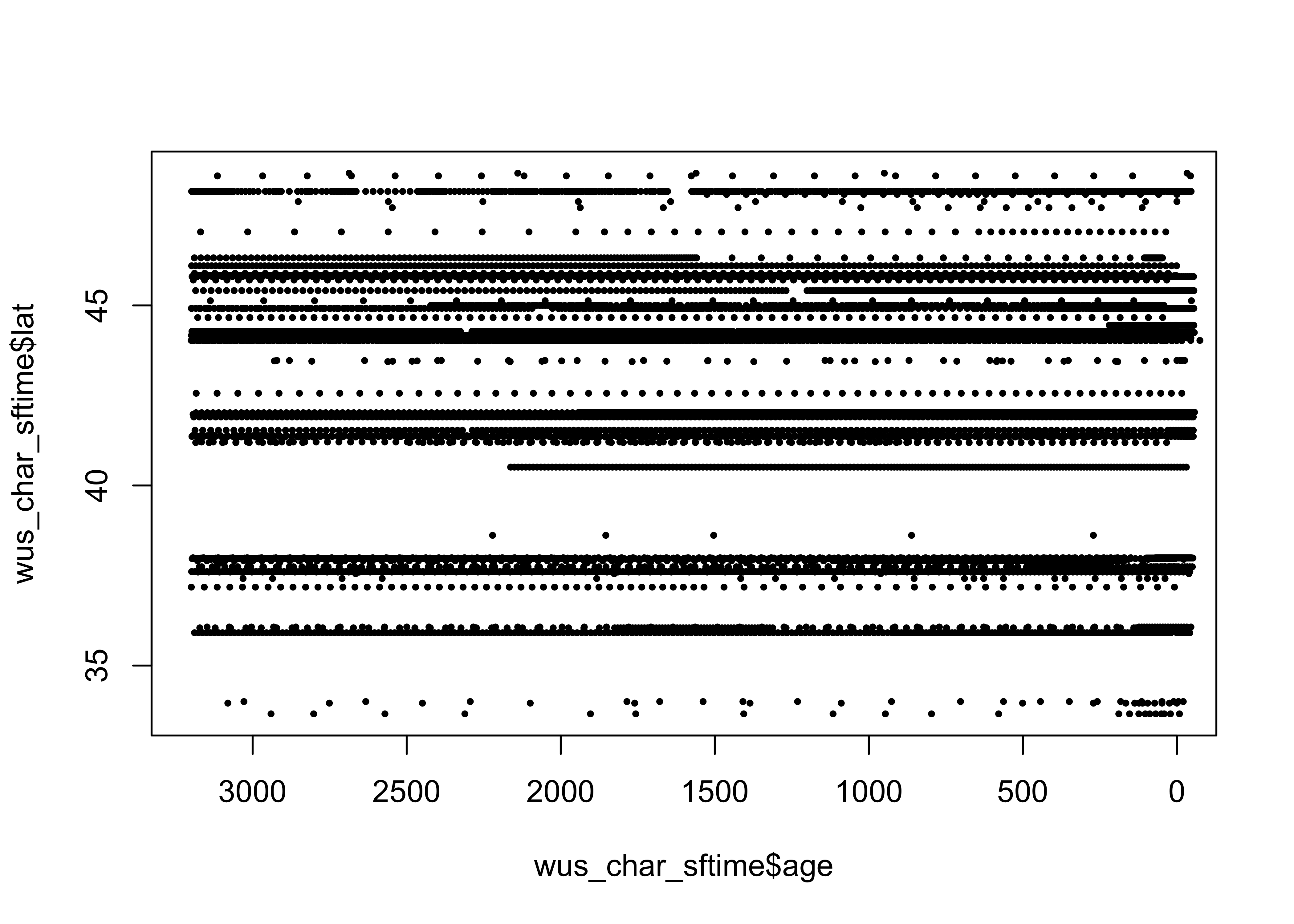
Note that data.frame is now an sf “POINT” object with explicit geometry (as well as a “time column”). Here’s a simple latitude by age plot ( Hovmöller diagram):

plot(wus_char_sftime$lat ~ wus_char_sftime$age, xlim = c(3200, 0), pch = 16, cex = 0.5)

Plot the locations of the sites.

# ggplot2 map of wus_char_sftime
ggplot()  +
  geom_sf(data = na2_sf, fill=NA) +
  geom_sf(data = wus_sf, fill=NA) +
  geom_point(aes(x = wus_char_sftime$lon, y = wus_char_sftime$lat), color = "red") +
  coord_sf(xlim = c(-130, -100), ylim = c(30, 50), expand = FALSE) +
  labs(title="Western U.S. High-Resolution Charcoal Records", x = "Longitude", y = "Latitude") + 
  theme_bw() + theme(legend.position="bottom")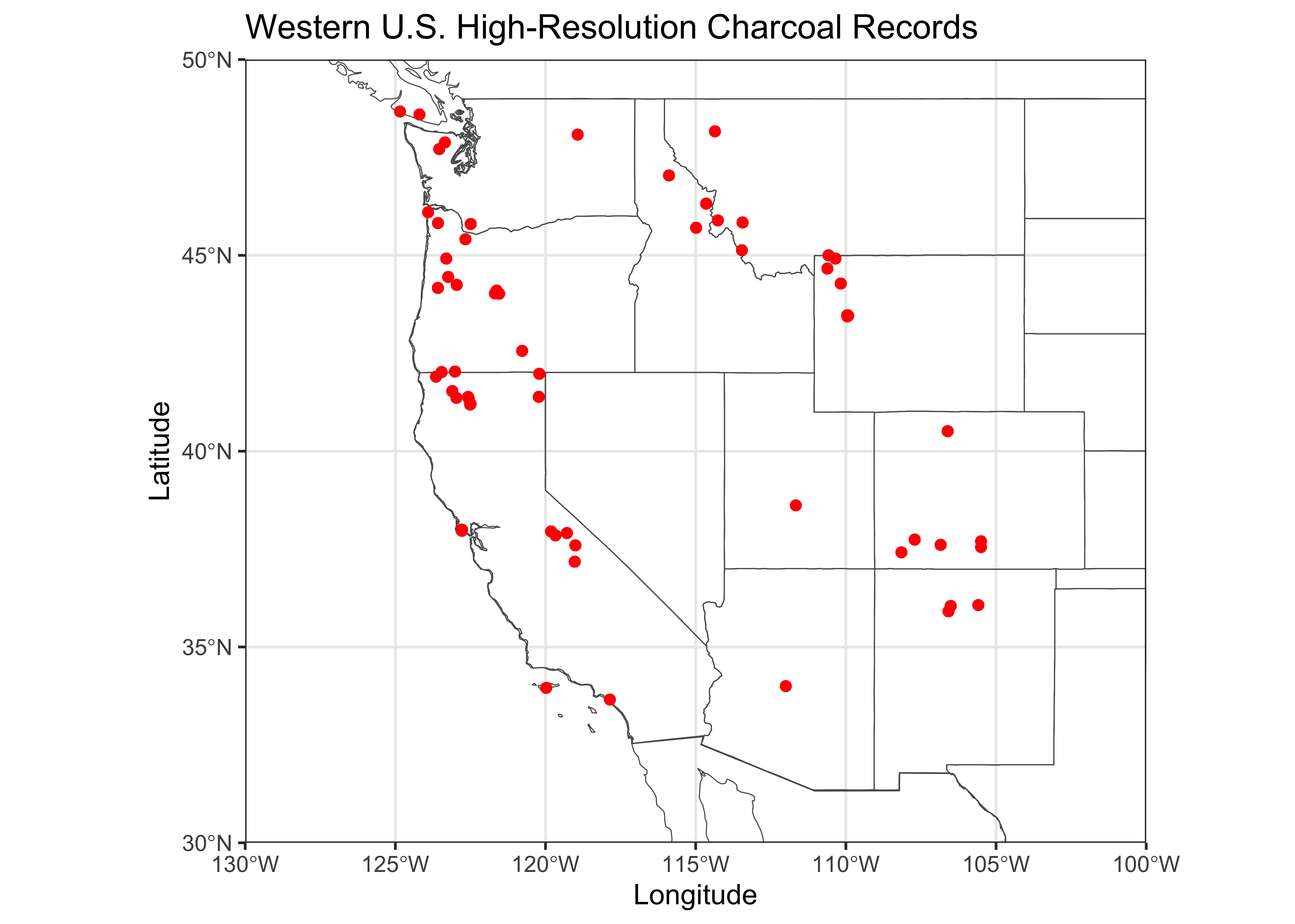

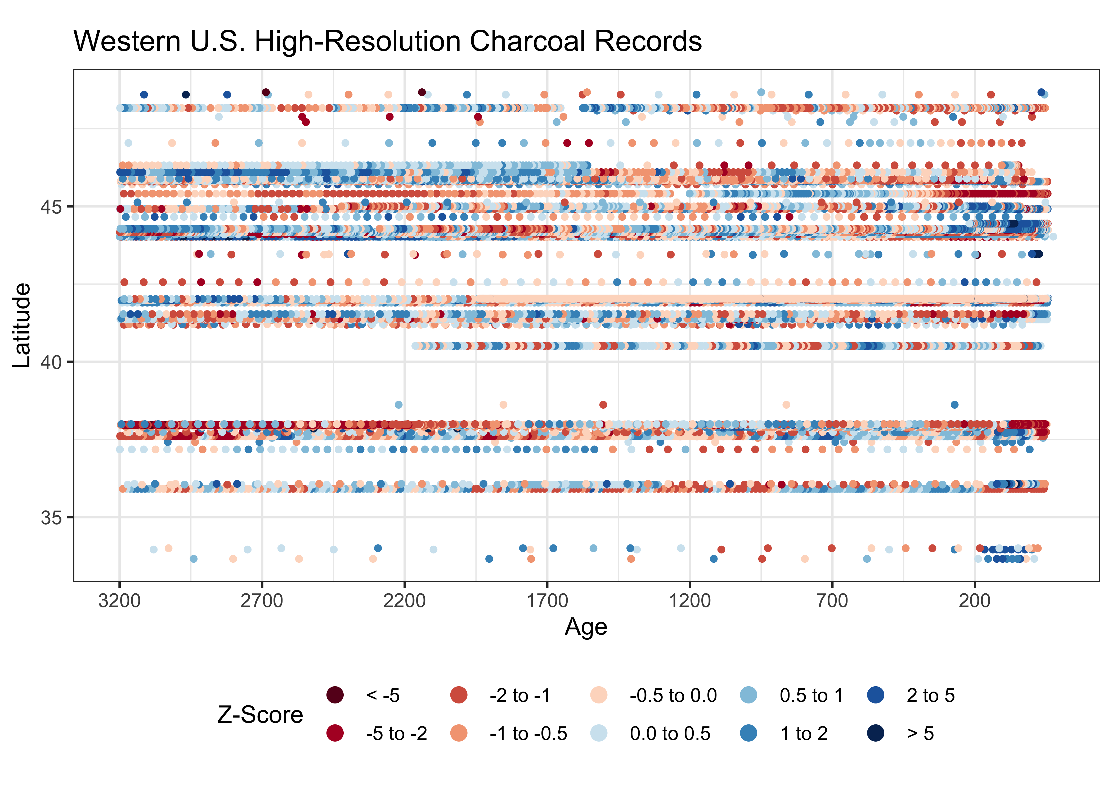
And here’s a better Hovmöller diagram:

# ggplot2 Hovmöller plots -- Year x Latitude

cutpts <- c(-99, -5, -2, -1, -0.5, 0.0, 0.5, 1, 2, 5, 99)
ztinflux_factor <- factor(findInterval(wus_char_sftime$ztinflux, cutpts))

ggplot() +
  scale_color_brewer(type = "div", palette = "RdBu", aesthetics = "color", direction = 0,
                     labels = c("< -5", "-5 to -2", "-2 to -1", "-1 to -0.5", "-0.5 to 0.0",
                                "0.0 to 0.5", "0.5 to 1", "1 to 2", "2 to 5", "> 5"),
                     name = "Z-Score") +
  geom_point(aes(x = wus_char_sftime$age, y = wus_char_sftime$lat, color = ztinflux_factor), size = 1) +
  scale_x_continuous(breaks = seq(3200, -100, -500), trans = "reverse") +
  scale_y_continuous(breaks = seq(30, 50, 5)) +
  labs(title="Western U.S. High-Resolution Charcoal Records", y = "Latitude", x = "Age", fill="Z-Scores Charcoal Influx") + 
  guides(color = guide_legend(override.aes = list(size=3))) +
  theme_bw() + theme(legend.position="bottom") + theme(aspect.ratio = 2/4)