1 Calculate long-term means and anomalies
2 Read the data
- 2.1 Read dimensions and attributes of the data set
- 2.2 Read the array
3 Why anomalies are useful
4 Long-term means
- 4.1 Set up for long-term mean calculation
- 4.2 Get long-term means
5 Get anomalies
6 Write netCDF files of the ltm’s and anomalies

NOTE: This page has been revised for Winter 2024, but may undergo further edits.

1 Calculate long-term means and anomalies

A common task in analyzing Earth-system science data is the calculation of “anomalies” or differences between individual months or years and some long-term average. This will produce two new data sets: 1) the long-term means (“ltm”) and 2) the anomalies (“anm”). The example here gets the long-term means and anomlies for the CRU TS 4.07 near-surface air temperature data set cru_ts4.07.1901.2022.tmp.dat. The data include monthly values for the interval 1901 - 2022, and the long-term means will be calculated for one of the commonly used base periods, 1961 - 1990.

2 Read the data

Load the necessary packages, and set paths and filenames:

# load the ncdf4 package
library(ncdf4)
library(CFtime)
library(lattice)
library(sf)

## Linking to GEOS 3.11.0, GDAL 3.5.3, PROJ 9.1.0; sf_use_s2() is TRUE

library(ggplot2)
library(RColorBrewer)

# set path and filename
ncpath <- "/Users/bartlein/Dropbox/DataVis/working/data/nc_files/"
ncname <- "cru_ts4.07.1901.2022.tmp.dat.nc"  
ncfname <- paste(ncpath, ncname, sep="")
dname <- "tmp"  # note: tmp means temperature (not temporary)

2.1 Read dimensions and attributes of the data set

Open the netCDF file (and list its contents), and read the dimension variables:

# open a netCDF file
ncin <- nc_open(ncfname)
print(ncin)

## File /Users/bartlein/Dropbox/DataVis/working/data/nc_files/cru_ts4.07.1901.2022.tmp.dat.nc (NC_FORMAT_CLASSIC):
## 
##      2 variables (excluding dimension variables):
##         float tmp[lon,lat,time]   
##             long_name: near-surface temperature
##             units: degrees Celsius
##             correlation_decay_distance: 1200
##             _FillValue: 9.96920996838687e+36
##             missing_value: 9.96920996838687e+36
##         int stn[lon,lat,time]   
##             description: number of stations contributing to each datum
##             _FillValue: -999
##             missing_value: -999
## 
##      3 dimensions:
##         lon  Size:720 
##             long_name: longitude
##             units: degrees_east
##         lat  Size:360 
##             long_name: latitude
##             units: degrees_north
##         time  Size:1464   *** is unlimited *** 
##             long_name: time
##             units: days since 1900-1-1
##             calendar: gregorian
## 
##     8 global attributes:
##         Conventions: CF-1.4
##         title: CRU TS4.07 Mean Temperature
##         institution: Data held at British Atmospheric Data Centre, RAL, UK.
##         source: Run ID = 2304141047. Data generated from:tmp.2304141039.dtb
##         history: Fri 14 Apr 11:30:51 BST 2023 : User f098 : Program makegridsauto.for called by update.for
##         references: Information on the data is available at http://badc.nerc.ac.uk/data/cru/
##         comment: Access to these data is available to any registered CEDA user.
##         contact: support@ceda.ac.uk

Read latitude, longitude, and time:

# get longitude and latitude
lon <- ncvar_get(ncin,"lon")
nlon <- dim(lon)
head(lon)

## [1] -179.75 -179.25 -178.75 -178.25 -177.75 -177.25

lat <- ncvar_get(ncin,"lat")
nlat <- dim(lat)
head(lat)

## [1] -89.75 -89.25 -88.75 -88.25 -87.75 -87.25

print(c(nlon,nlat))

## [1] 720 360

# get time
time <- ncvar_get(ncin,"time")
tunits <- ncatt_get(ncin,"time","units")
nt <- dim(time)

nm <- 12
ny <- nt/nm

Decode the time variable (but don’t overwrite anything):

# decode time
cf <- CFtime(tunits$value, calendar = "proleptic_gregorian", time) # convert time to CFtime class
timestamps <- CFtimestamp(cf) # get character-string times
time_cf <- CFparse(cf, timestamps) # parse the string into date components
# list a few values
head(time_cf)

##   year month day hour minute second    tz offset
## 1 1901     1  16    0      0      0 00:00    380
## 2 1901     2  15    0      0      0 00:00    410
## 3 1901     3  16    0      0      0 00:00    439
## 4 1901     4  16    0      0      0 00:00    470
## 5 1901     5  16    0      0      0 00:00    500
## 6 1901     6  16    0      0      0 00:00    531

Note that the day variable value is 16, the middle day of each month.

2.2 Read the array

Read the data, and get variable and global attributes:

# get temperature
tmp_array <- ncvar_get(ncin,dname)
dlname <- ncatt_get(ncin,dname,"long_name")
dunits <- ncatt_get(ncin,dname,"units")
fillvalue <- ncatt_get(ncin,dname,"_FillValue")
dim(tmp_array)

## [1]  720  360 1464

# get global attributes
title <- ncatt_get(ncin,0,"title")
institution <- ncatt_get(ncin,0,"institution")
datasource <- ncatt_get(ncin,0,"source")
references <- ncatt_get(ncin,0,"references")
history <- ncatt_get(ncin,0,"history")
Conventions <- ncatt_get(ncin,0,"Conventions")

Close the netCDF data set.

# close the netCDF file
nc_close(ncin)

Replace netCDF fill values with R NA’s

# replace netCDF fill values with NA's
tmp_array[tmp_array==fillvalue$value] <- NA
length(na.omit(as.vector(tmp_array[,,1])))

## [1] 67420

3 Why anomalies are useful

There several reasons why anomalies (or deviations from a particular, say, month from the long-term mean values for that month of the year) are useful. The main motivation is that for many climate variables, like temperature, the spatial variations of climate are much greater than temporal variations, and will dominate the map patterns in comparing any two months (say, one at the beginning of the 20th Century and one at the end). By subtracting the long-term mean values (over, say, a 30-year period), which will also contain the high spatial variability of climate, the temporal difference between the two months will become evident. Another reason for looking at anomalies, is that features that anomaly maps reveal can be regarded as entities in their own right, and correlated among variables, while observing their evolution over time.

To get a idea of the first motivation, get the values for the first observation in the data set, January 1901, and get a quick levelplot:

# levelplot of the slice
n <- 1
grid <- expand.grid(lon=lon, lat=lat)
cutpts <- c(-50,-40,-30,-20,-10,0,10,20,30,40,50)
levelplot(tmp_array[,, n] ~ lon * lat, data=grid, at=cutpts, cuts=11, pretty=T, 
  col.regions=(rev(brewer.pal(10,"RdBu"))), main = "Jan 1901")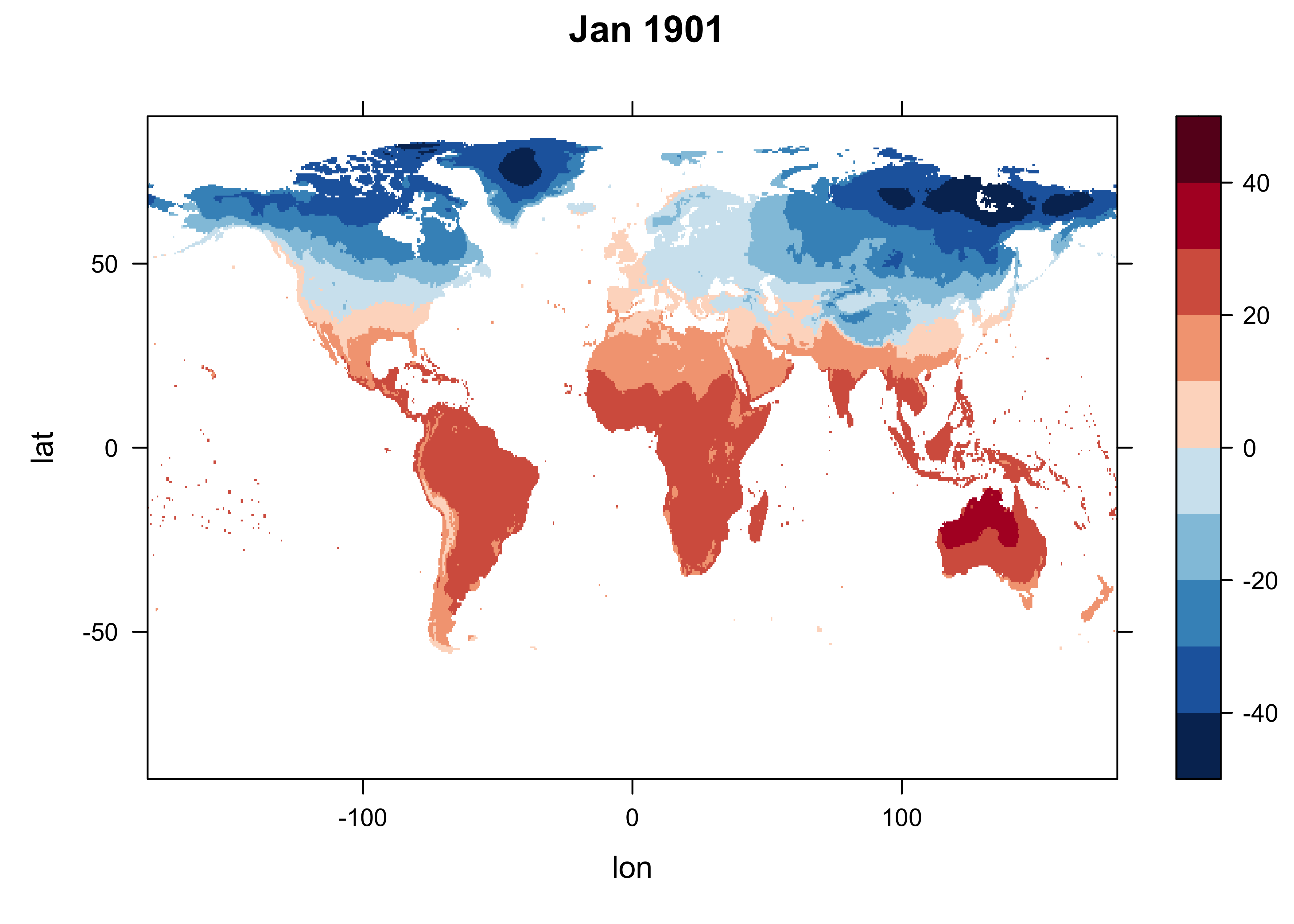

Now get a single slice of the array, for, January 2022 (n = 1453), and make a quick levelplot.

# levelplot of the slice
n <- 1464
grid <- expand.grid(lon=lon, lat=lat)
cutpts <- c(-50,-40,-30,-20,-10,0,10,20,30,40,50)
levelplot(tmp_array[,, n] ~ lon * lat, data=grid, at=cutpts, cuts=11, pretty=T, 
  col.regions=(rev(brewer.pal(10,"RdBu"))), main = "Jan 2022")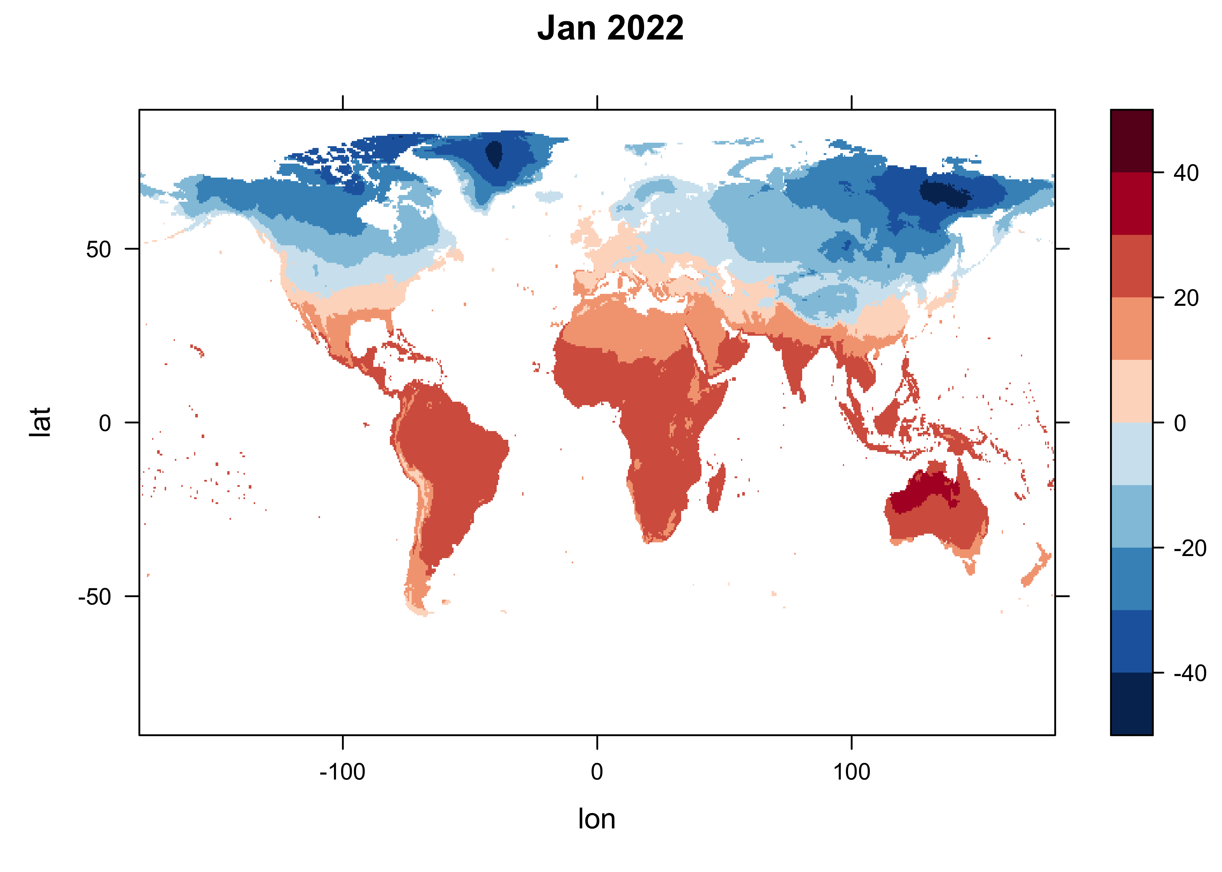

The maps are quite similar, despite the fact that we know significant climate change has take place over this interval.

4 Long-term means

4.1 Set up for long-term mean calculation

Get the indices for the beginning and end of the base period, and save them as a string.

# get beginning obs of base period
begyr <- 1961; endyr <- 1990; nyrs <- endyr - begyr + 1
begobs <- ((begyr - time_cf$year[1]) * nm) + 1
endobs <- ((endyr - time_cf$year[1] + 1) * nm)
base_period <- paste(as.character(begyr)," - ", as.character(endyr), sep="")
print(c(begyr, endyr, begobs, endobs, base_period))

## [1] "1961"        "1990"        "721"         "1080"        "1961 - 1990"

Get a levelplot of the first observation in the base period.

# levelplot of begobs
tmp_slice <- tmp_array[,, begobs]
grid <- expand.grid(lon=lon, lat=lat)
cutpts <- c(-50,-40,-30,-20,-10,0,10,20,30,40,50)
levelplot(tmp_slice ~ lon * lat, data=grid, at=cutpts, cuts=11, pretty=T, 
          col.regions=(rev(brewer.pal(10,"RdBu"))))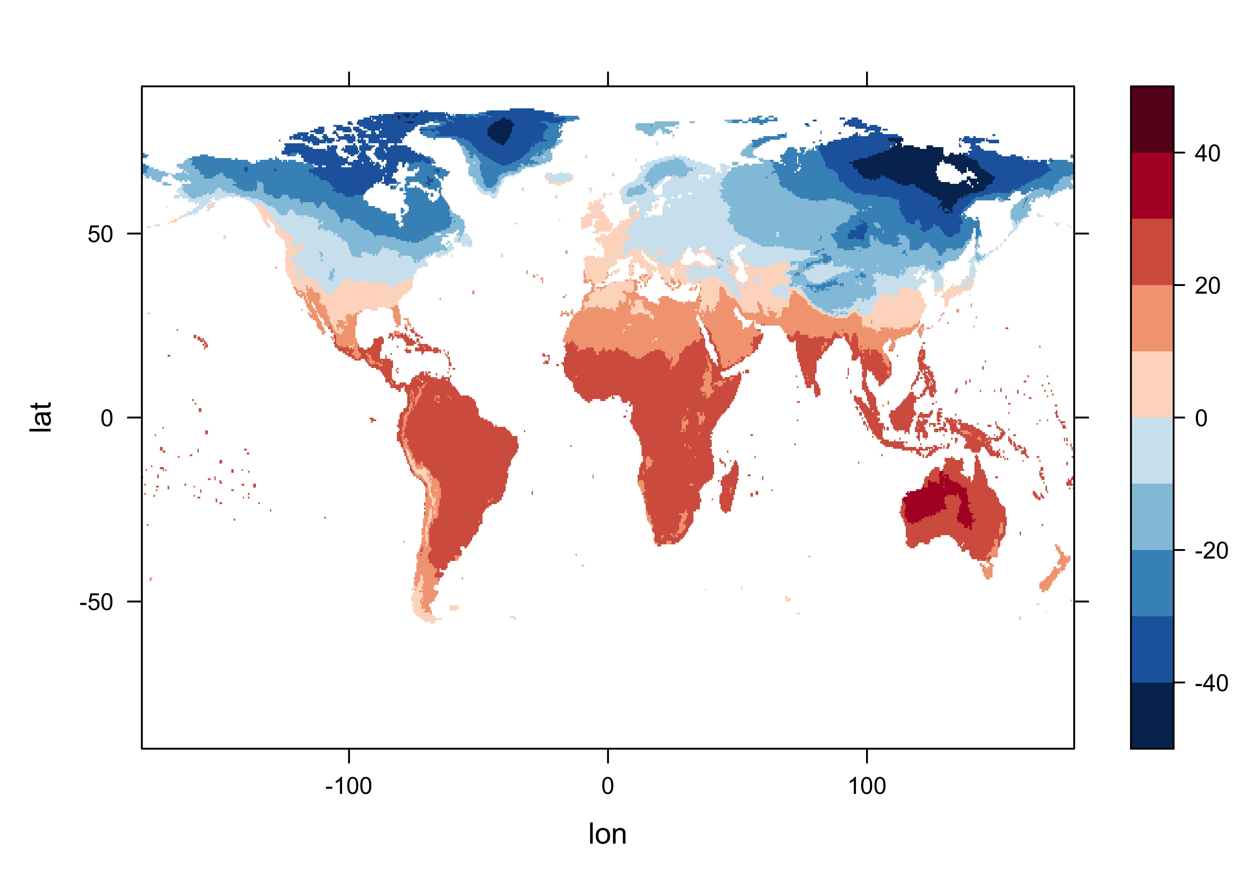

Create a new array with just the base period data in it.

# base-period array
tmp_array_base <- array(dim = c(nlon, nlat, nyrs * nm))
dim(tmp_array_base)

## [1] 720 360 360

tmp_array_base <- tmp_array[,, begobs:endobs]

Get a levelplot of the first time-slice of that, which should match the previous plot

# levelplot of tmp_array_base
tmp_slice <- tmp_array_base[,, 1]
grid <- expand.grid(lon=lon, lat=lat)
cutpts <- c(-50,-40,-30,-20,-10,0,10,20,30,40,50)
levelplot(tmp_slice ~ lon * lat, data=grid, at=cutpts, cuts=11, pretty=T, 
          col.regions=(rev(brewer.pal(10,"RdBu"))))

4.2 Get long-term means

The long-term means are calculated by looping over the grid cells and months.

# long-term means
tmp_ltm <- array(NA, dim = c(nlon, nlat, nm))
dim(tmp_ltm)

## [1] 720 360  12

for (j in 1:nlon) {
  for (k in 1:nlat) {
    if (!is.na(tmp_array_base[j, k, 1])) {
      for (m in 1:nm)
        tmp_ltm[j, k, m] <- mean(tmp_array_base[j, k, seq(m, (m + nm*nyrs - 1), by=nm)])
    }
  }
}

Levelplot of the January long-term means:

# levelplot of tmp_ltm
tmp_slice <- tmp_ltm[,, 1]
grid <- expand.grid(lon=lon, lat=lat)
cutpts <- c(-50,-40,-30,-20,-10,0,10,20,30,40,50)
levelplot(tmp_slice ~ lon * lat, data=grid, at=cutpts, cuts=11, pretty=T, 
          col.regions=(rev(brewer.pal(10,"RdBu"))))

A {ggplot2} multi-panel maps of the long-term means can be made by turning the tmp_ltm array into a dataframe as follow:

# unwrap the array to a long vector, stacking the months
tmp_ltm_vector <- as.vector(tmp_ltm)
lonlat <- as.matrix(expand.grid(lon, lat))
# month names
np <- dim(tmp_ltm)[1] * dim(tmp_ltm)[2]
month <- c(rep("Jan", np), rep("Feb", np), rep("Mar", np), rep("Apr", np), rep("May", np), rep("Jun", np),
  rep("Jul", np), rep("Aug", np), rep("Sep", np), rep("Oct", np), rep("Nov", np), rep("Dec", np))
# make the dataframe
tmp_ltm_df <- data.frame(lonlat[,1], lonlat[,2], tmp_ltm_vector, month)
names(tmp_ltm_df) <- c("lon", "lat", "tmp_ltm", "month")

Get a world outline:

# world_sf
world_sf <- st_as_sf(maps::map("world", plot = FALSE, fill = TRUE))
world_otl_sf <- st_geometry(world_sf)

Make the map.

# ggplot2 map of tmp_ltm
ggplot() + 
  geom_tile(data = tmp_ltm_df, aes(x = lon, y = lat, fill = tmp_ltm)) +
  geom_sf(data = world_otl_sf, col = "black", fill = NA) +
  # geom_sf(data = grat_otl, col = "gray80", lwd = 0.5, lty = 3) +
  coord_sf(xlim = c(-180, +180), ylim = c(-90, 90), expand = FALSE) +
  facet_wrap(~factor(month, levels = 
    c("Dec", "Jan", "Feb", "Mar", "Apr", "May", "Jun", "Jul", "Aug", "Sep", "Oct", "Nov")), nrow = 4, ncol = 3) +
  scale_fill_gradient2(low = "darkblue", mid="white", high = "darkred", midpoint = 0.0) +
  # scale_y_continuous(breaks = seq(-90, 90, 90), expand = c(0,0)) +  # removes whitespace within panels
  # scale_x_continuous(breaks = seq(-180, 180, 90), expand = c(0,0)) +
  scale_y_continuous(breaks = seq(-90, 90, 30)) +
  scale_x_continuous(breaks = seq(-180, 180, 60)) +
  labs(title="CRU TS 4.07 Long-term mean temperature", fill="K") + 
  theme_bw() + theme(strip.text = element_text(size = 6))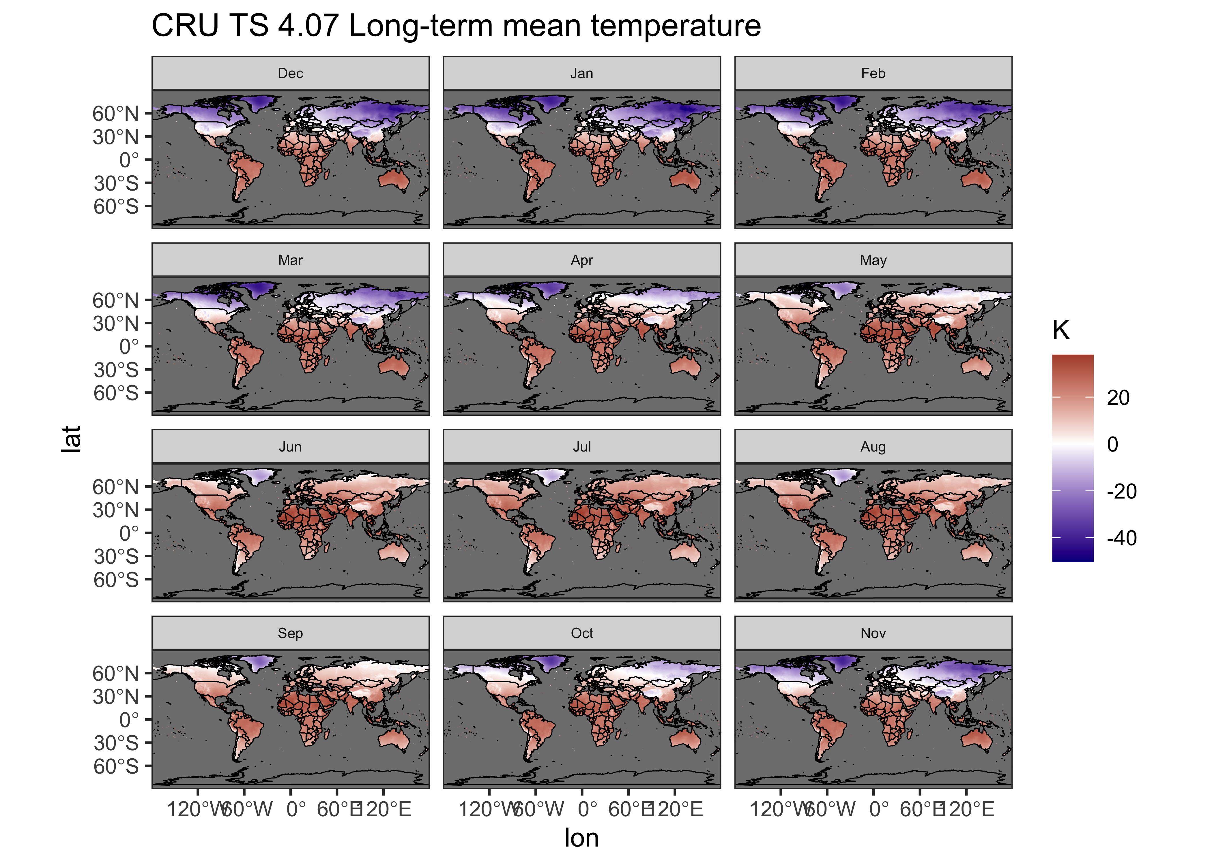

Note the rearrangement of the months (“Dec”, …, “Nov”) in the factor() function. This places the standard meteorological seasons, DJF (December, January, February), MAM, JJA, SON on each row of the plot.

5 Get anomalies

The anomalies are obtaimed for each grid point by simply expanding the twelve ltm values (one for each month of the year) over the ny years of the record, and then differencing. In this way, the anomaly for each January in the record is the difference between the “absolute” (but not “absolute value” (abs())) or observed value, and the January long-term mean.

# anomalies
tmp_anm <- array(NA, dim = c(nlon, nlat, nt))
tmp_anm <- tmp_array - rep(tmp_ltm, ny)

Get a levelplot of an anomaly. Note the different cutpoints.

# levelplot of tmp_ltm
tmp_slice <- tmp_anm[,, 1]
grid <- expand.grid(lon=lon, lat=lat)
cutpts <- c(-10,-5,-2,-1,-0.5,0,0.5,1,2,5,10)
levelplot(tmp_slice ~ lon * lat, data=grid, at=cutpts, cuts=11, pretty=T, 
          col.regions=(rev(brewer.pal(10,"RdBu"))))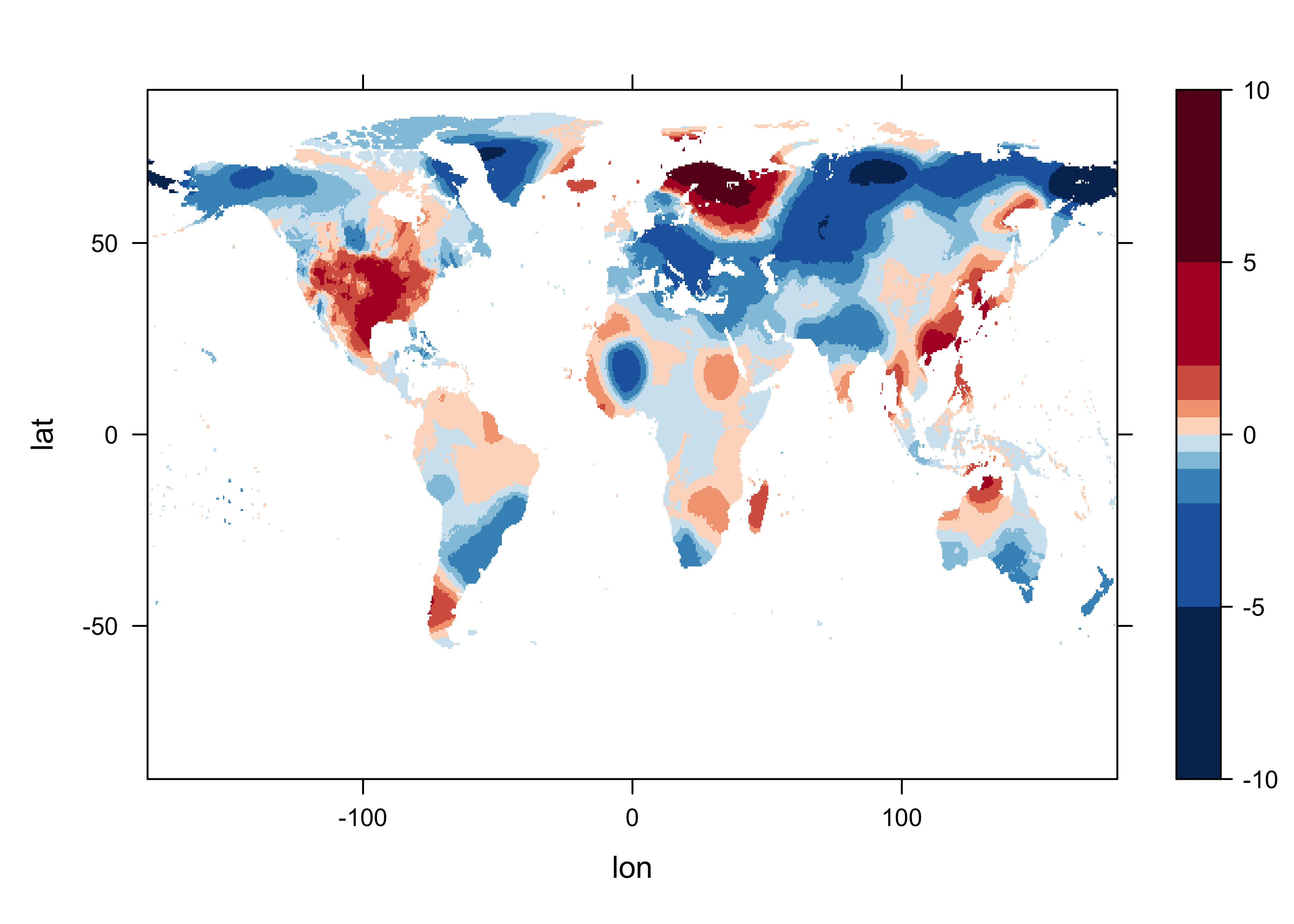

6 Write netCDF files of the ltm’s and anomalies

Write out netCDF files of the long-term means and anomalies in the usual way.

# netCDF file of ltm's

# path and file name, set dname
ncpath <- "/Users/bartlein/Projects/RESS/data/nc_files/"
ncname <- "cru_ts4.07.1961.1990.tmp.ltm.nc"   
ncfname <- paste(ncpath, ncname, sep="")
dname <- "tmp_ltm"  # note: tmp means temperature (not temporary)

# get time values for output
time_out <- time[(begobs + (nyrs/2)*nm):(begobs + (nyrs/2)*nm + nm - 1)]

# recode NA's to fill_values
tmp_ltm[is.na(tmp_ltm)] <- fillvalue$value

# create and write the netCDF file -- ncdf4 version
# define dimensions
londim <- ncdim_def("lon","degrees_east",as.double(lon)) 
latdim <- ncdim_def("lat","degrees_north",as.double(lat)) 
timedim <- ncdim_def("time",tunits$value,as.double(time_out))

# define variables
dlname <- "near-surface air temperature long-term mean"
tmp_def <- ncvar_def("tmp_ltm","degrees Celsius",list(londim,latdim,timedim),fillvalue$value,dlname,prec="single")

# create netCDF file and put arrays
ncout <- nc_create(ncfname,tmp_def,force_v4=TRUE)

# put variables
ncvar_put(ncout,tmp_def,tmp_ltm)

# put additional attributes into dimension and data variables
ncatt_put(ncout,"lon","axis","X") #,verbose=FALSE) #,definemode=FALSE)
ncatt_put(ncout,"lat","axis","Y")
ncatt_put(ncout,"time","axis","T")
ncatt_put(ncout,"tmp_ltm","base_period", base_period)

# add global attributes
ncatt_put(ncout,0,"title",title$value)
ncatt_put(ncout,0,"institution",institution$value)
ncatt_put(ncout,0,"source",datasource$value)
ncatt_put(ncout,0,"references",references$value)
history <- paste("P.J. Bartlein", date(), sep=", ")
ncatt_put(ncout,0,"history",history)
ncatt_put(ncout,0,"Conventions",Conventions$value)

# Get a summary of the created file:
ncout

# close the file, writing data to disk
nc_close(ncout)

# netCDF file of anomalies

# path and file name, set dname
ncpath <- "/Users/bartlein/Projects/RESS/data/nc_files/"
ncname <- "cru_ts4.07.1901.2022.tmp.anm.nc"   
ncfname <- paste(ncpath, ncname, sep="")
dname <- "tmp_anm"  # note: tmp means temperature (not temporary)

# recode NA's to fill_values
tmp_anm[is.na(tmp_anm)] <- fillvalue$value

# create and write the netCDF file -- ncdf4 version
# define dimensions
londim <- ncdim_def("lon","degrees_east",as.double(lon)) 
latdim <- ncdim_def("lat","degrees_north",as.double(lat)) 
timedim <- ncdim_def("time",tunits$value,as.double(time))

# define variables
dlname <- "near-surface air temperature anomalies"
tmp_def <- ncvar_def("tmp_anm","degrees Celsius",list(londim,latdim,timedim),fillvalue$value,dlname,prec="single")

# create netCDF file and put arrays
ncout <- nc_create(ncfname,tmp_def,force_v4=TRUE)

# put variables
ncvar_put(ncout,tmp_def,tmp_anm)

# put additional attributes into dimension and data variables
ncatt_put(ncout,"lon","axis","X") #,verbose=FALSE) #,definemode=FALSE)
ncatt_put(ncout,"lat","axis","Y")
ncatt_put(ncout,"time","axis","T")
ncatt_put(ncout,"tmp_anm","base_period", base_period)

# add global attributes
ncatt_put(ncout,0,"title",title$value)
ncatt_put(ncout,0,"institution",institution$value)
ncatt_put(ncout,0,"source",datasource$value)
ncatt_put(ncout,0,"references",references$value)
history <- paste("P.J. Bartlein", date(), sep=", ")
ncatt_put(ncout,0,"history",history)
ncatt_put(ncout,0,"Conventions",Conventions$value)

# Get a summary of the created file:
ncout

# close the file, writing data to disk
nc_close(ncout)

Long-term means and anomalies