Maps (2)
NOTE: This page has been revised for Winter 2024, but may undergo further edits.
1 A second example
This second example illustrates the creating of a base map for North
America that conforms to the projection used for the
na10km_v2 data, a data set of present-day climate that
accompanies a packrat-midden database: Strickland, L.E., Thompson, R.S.,
Shafer, S.L., Bartlein, P.J., Pelltier, R.T., Anderson, K.H., Schumann,
R.R., McFadden, A.K., 2024. Plant macrofossil data for 48-0 ka in the
USGS North American Packrat Midden Database, version 5.0. Scientific
Data 11, 68. [https://www.nature.com/articles/s41597-023-02616-y].
As before, Natural Earth shapefiles are read and projected,
this time using a Lambert Azimuthal Equal-Area projection, and trimmed
to the appropriate region.
1.1 Read the Natural Earth shapefiles
Load the appropriate packages.
Set the shapefile names, including those for global coastlines, adminstrative units (borders). (Note that these are smaller-spatial/larger-cartrographic resolution shapefiles, more appropriate for continental-scale as opposed to global-scale mapping.) Set the filenames:
# read Natural Earth shapefiles
shape_path <- "/Users/bartlein/Projects/RESS/data/RMaps/source/"
coast_shapefile <- paste(shape_path, "ne_10m_coastline/ne_10m_coastline.shp", sep="")
admin0_shapefile <- paste(shape_path, "ne_10m_admin_0_countries/ne_10m_admin_0_countries.shp", sep="")
admin1_shapefile <- paste(shape_path,
        "ne_10m_admin_1_states_provinces_lakes/ne_10m_admin_1_states_provinces_lakes.shp", sep="")
lakes_shapefile <- paste(shape_path, "ne_10m_lakes/ne_10m_lakes.shp", sep="")
grat15_shapefile <- paste(shape_path, "ne_10m_graticules_all/ne_10m_graticules_15.shp", sep="")
As before, query geometry types to compose object names:
# query geometry type
coast_geometry <- as.character(st_geometry_type(st_read(coast_shapefile), by_geometry = FALSE))
## Reading layer `ne_10m_coastline' from data source
## `/Users/bartlein/Projects/RESS/data/RMaps/source/ne_10m_coastline/ne_10m_coastline.shp'
## using driver `ESRI Shapefile'
## Simple feature collection with 4132 features and 2 fields
## Geometry type: LINESTRING
## Dimension: XY
## Bounding box: xmin: -180 ymin: -85.22194 xmax: 180 ymax: 83.6341
## Geodetic CRS: WGS 84## [1] "LINESTRING"Read and plot the shapefiles. At a higher spatial resolution, these files will take more time to load. (Note: summary output is suppressed)
# read shapefiles
coast_lines_sf <- st_read(coast_shapefile) # note geometry type MULTILINESTRING
plot(st_geometry(coast_lines_sf), col="gray50")
admin0_poly_sf <- st_read(admin0_shapefile) # note:  geometry type MULTIPOLYGON
plot(st_geometry(admin0_poly_sf), col="gray70", border="red", add = TRUE)
admin1_poly_sf <- st_read(admin1_shapefile) # note:  geometry type MULTIPOLYGON
plot(st_geometry(admin1_poly_sf), col="gray70", border="pink", add = TRUE)
lakes_poly_sf <- st_read(lakes_shapefile) # note:  geometry type POLYGON
plot(st_geometry(lakes_poly_sf), col="blue", add = TRUE)
grat15_lines_sf <- st_read(grat15_shapefile) # note:  geometry type LINESTRING
plot(st_geometry(grat15_lines_sf), col="gray50", add = TRUE)

# filter out the small lakes
lrglakes_poly_sf <- lakes_poly_sf[as.numeric(lakes_poly_sf$scalerank) <= 2 ,]
plot(lrglakes_poly_sf, bor="purple", add=TRUE)
## Warning in plot.sf(lrglakes_poly_sf, bor = "purple", add = TRUE): ignoring all but the first attribute
Take a look at the admin1_poly dataframe, to figure out
the codes for Canadian and U.S. provincial and state borders.
## Simple feature collection with 6 features and 65 fields
## Geometry type: MULTIPOLYGON
## Dimension:     XY
## Bounding box:  xmin: -70.06241 ymin: -18.0314 xmax: 74.89231 ymax: 60.48078
## Geodetic CRS:  WGS 84
##   scalerank      featurecla LABELRANK     SOVEREIGNT SOV_A3 ADM0_DIF LEVEL              TYPE       ADMIN
## 1         3 Admin-0 country         5    Netherlands    NL1        1     2           Country       Aruba
## 2         0 Admin-0 country         3    Afghanistan    AFG        0     2 Sovereign country Afghanistan
## 3         0 Admin-0 country         3         Angola    AGO        0     2 Sovereign country      Angola
## 4         3 Admin-0 country         6 United Kingdom    GB1        1     2        Dependency    Anguilla
## 5         0 Admin-0 country         6        Albania    ALB        0     2 Sovereign country     Albania
## 6         3 Admin-0 country         6        Finland    FI1        1     2           Country       Aland
##   ADM0_A3 GEOU_DIF     GEOUNIT GU_A3 SU_DIF     SUBUNIT SU_A3 BRK_DIFF        NAME     NAME_LONG BRK_A3
## 1     ABW        0       Aruba   ABW      0       Aruba   ABW        0       Aruba         Aruba    ABW
## 2     AFG        0 Afghanistan   AFG      0 Afghanistan   AFG        0 Afghanistan   Afghanistan    AFG
## 3     AGO        0      Angola   AGO      0      Angola   AGO        0      Angola        Angola    AGO
## 4     AIA        0    Anguilla   AIA      0    Anguilla   AIA        0    Anguilla      Anguilla    AIA
## 5     ALB        0     Albania   ALB      0     Albania   ALB        0     Albania       Albania    ALB
## 6     ALD        0       Aland   ALD      0       Aland   ALD        0       Aland Aland Islands    ALD
##      BRK_NAME BRK_GROUP ABBREV POSTAL                    FORMAL_EN FORMAL_FR NOTE_ADM0 NOTE_BRK
## 1       Aruba      <NA>  Aruba     AW                        Aruba      <NA>     Neth.     <NA>
## 2 Afghanistan      <NA>   Afg.     AF Islamic State of Afghanistan      <NA>      <NA>     <NA>
## 3      Angola      <NA>   Ang.     AO  People's Republic of Angola      <NA>      <NA>     <NA>
## 4    Anguilla      <NA>   Ang.     AI                         <NA>      <NA>      U.K.     <NA>
## 5     Albania      <NA>   Alb.     AL          Republic of Albania      <NA>      <NA>     <NA>
## 6       Aland      <NA>  Aland     AI                Åland Islands      <NA>      Fin.     <NA>
##     NAME_SORT NAME_ALT MAPCOLOR7 MAPCOLOR8 MAPCOLOR9 MAPCOLOR13  POP_EST GDP_MD_EST POP_YEAR LASTCENSUS
## 1       Aruba     <NA>         4         2         2          9   103065     2258.0      -99       2010
## 2 Afghanistan     <NA>         5         6         8          7 28400000    22270.0      -99       1979
## 3      Angola     <NA>         3         2         6          1 12799293   110300.0      -99       1970
## 4    Anguilla     <NA>         6         6         6          3    14436      108.9      -99        -99
## 5     Albania     <NA>         1         4         1          6  3639453    21810.0      -99       2001
## 6       Aland     <NA>         4         1         4          6    27153     1563.0      -99        -99
##   GDP_YEAR                    ECONOMY              INCOME_GRP WIKIPEDIA FIPS_10_ ISO_A2 ISO_A3 ISO_N3
## 1      -99       6. Developing region 2. High income: nonOECD       -99       AA     AW    ABW    533
## 2      -99  7. Least developed region           5. Low income       -99       AF     AF    AFG    004
## 3      -99  7. Least developed region  3. Upper middle income       -99       AO     AO    AGO    024
## 4      -99       6. Developing region  3. Upper middle income       -99       AV     AI    AIA    660
## 5      -99       6. Developing region  4. Lower middle income       -99       AL     AL    ALB    008
## 6      -99 2. Developed region: nonG7    1. High income: OECD       -99      -99     AX    ALA    248
##   UN_A3 WB_A2 WB_A3   WOE_ID WOE_ID_EH                   WOE_NOTE ADM0_A3_IS ADM0_A3_US ADM0_A3_UN
## 1   533    AW   ABW 23424736  23424736 Exact WOE match as country        ABW        ABW        -99
## 2   004    AF   AFG 23424739  23424739 Exact WOE match as country        AFG        AFG        -99
## 3   024    AO   AGO 23424745  23424745 Exact WOE match as country        AGO        AGO        -99
## 4   660   -99   -99 23424751  23424751 Exact WOE match as country        AIA        AIA        -99
## 5   008    AL   ALB 23424742  23424742 Exact WOE match as country        ALB        ALB        -99
## 6   248   -99   -99 12577865  12577865 Exact WOE match as country        ALA        ALD        -99
##   ADM0_A3_WB     CONTINENT REGION_UN       SUBREGION                 REGION_WB NAME_LEN LONG_LEN
## 1        -99 North America  Americas       Caribbean Latin America & Caribbean        5        5
## 2        -99          Asia      Asia   Southern Asia                South Asia       11       11
## 3        -99        Africa    Africa   Middle Africa        Sub-Saharan Africa        6        6
## 4        -99 North America  Americas       Caribbean Latin America & Caribbean        8        8
## 5        -99        Europe    Europe Southern Europe     Europe & Central Asia        7        7
## 6        -99        Europe    Europe Northern Europe     Europe & Central Asia        5       13
##   ABBREV_LEN TINY HOMEPART                       geometry
## 1          5    4      -99 MULTIPOLYGON (((-69.99694 1...
## 2          4  -99        1 MULTIPOLYGON (((71.0498 38....
## 3          4  -99        1 MULTIPOLYGON (((11.73752 -1...
## 4          4  -99      -99 MULTIPOLYGON (((-63.03767 1...
## 5          4  -99        1 MULTIPOLYGON (((19.74777 42...
## 6          5    5      -99 MULTIPOLYGON (((20.92018 59...
The approprate code to extract the U.S. and Canada data is
admin1_poly$sr_sov_a3 == "CAN" and
admin1_poly$sr_sov_a3 == "US1". Extract the borders, and
plot the resulting shapefiles.
# extract US and Canada boundaries
can_poly_sf <- admin1_poly_sf[admin1_poly_sf$sov_a3 == "CAN" ,]
us_poly_sf <- admin1_poly_sf[admin1_poly_sf$sov_a3 == "US1",]
plot(st_geometry(coast_lines_sf))
plot(st_geometry(can_poly_sf), border = "red", add=TRUE)
plot(st_geometry(us_poly_sf), border = "blue", add=TRUE)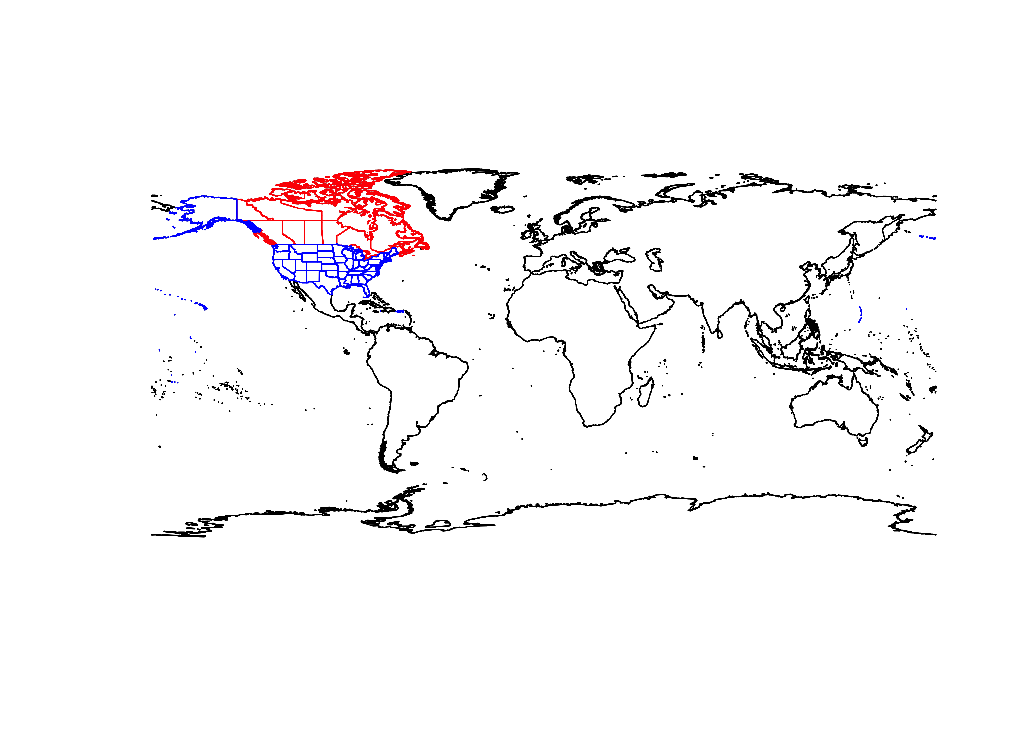
Convert the U.S. and Canada polygons to
MULTILINESTRINGS:
1.2 Project the shape files
Set the proj4string value and the coordinate reference
system for the na10km_v2 grid:
# Lambert Azimuthal Equal Area
na_proj4string <- "+proj=laea +lon_0=-100 +lat_0=50 +x_0=0 +y_0=0 +ellps=WGS84 +datum=WGS84 +units=m +no_defs"
na_crs = st_crs(na_proj4string)
Project the various shapefiles (and plot the coastlines as an example):
coast_lines_proj <- st_transform(coast_lines_sf, crs = na_crs)
admin0_poly_proj <- st_transform(admin0_poly_sf, crs = na_crs)
admin0_lines_proj <- st_transform(admin0_lines_sf, crs = na_crs)
admin1_poly_proj <- st_transform(admin1_poly_sf, crs = na_crs)
lakes_poly_proj <- st_transform(lakes_poly_sf, crs = na_crs)
lrglakes_poly_proj <- st_transform(lrglakes_poly_sf, crs = na_crs)
can_poly_proj <- st_transform(can_poly_sf, crs = na_crs)
us_poly_proj <- st_transform(us_poly_sf, crs = na_crs)
can_lines_proj <- st_transform(can_lines_sf, crs = na_crs)
us_lines_proj <- st_transform(us_lines_sf, crs = na_crs)
grat15_lines_proj <- st_transform(grat15_lines_sf, crs = na_crs)plot(st_geometry(admin0_lines_proj), col = "gray70")
plot(st_geometry(coast_lines_proj), col = "black", add=TRUE)
plot(st_geometry(grat15_lines_proj), col = "gray70", add=TRUE)
Define a bounding box for trimming the polygon and line shape files
to the area covered by the na10km_v2 grid. The extent of the area is
known from the definition of the grid, but could also be determined by
reading an na10km_v2 netCDF file. The projected admin shape
files are quite complicated, and create “topology exception errors”.
These can be fixed using an approach discussed on StackExchange [link]
# North America Bounding box (coords in metres)
na10km_bb <- st_bbox(c(xmin = -5770000, ymin = -4510000, xmax = 5000000, ymax = 4480000), crs = na_proj4string)
na10km_bb <- st_as_sfc(na10km_bb)
Clip or trim the coastlines to the na10km_bb
boundary-box object, using the st_intersection()
function:
# clip the projected objects to the na10km_bb
na10km_coast_lines_proj <- st_intersection(coast_lines_proj, na10km_bb)
## Warning: attribute variables are assumed to be spatially constant throughout all geometries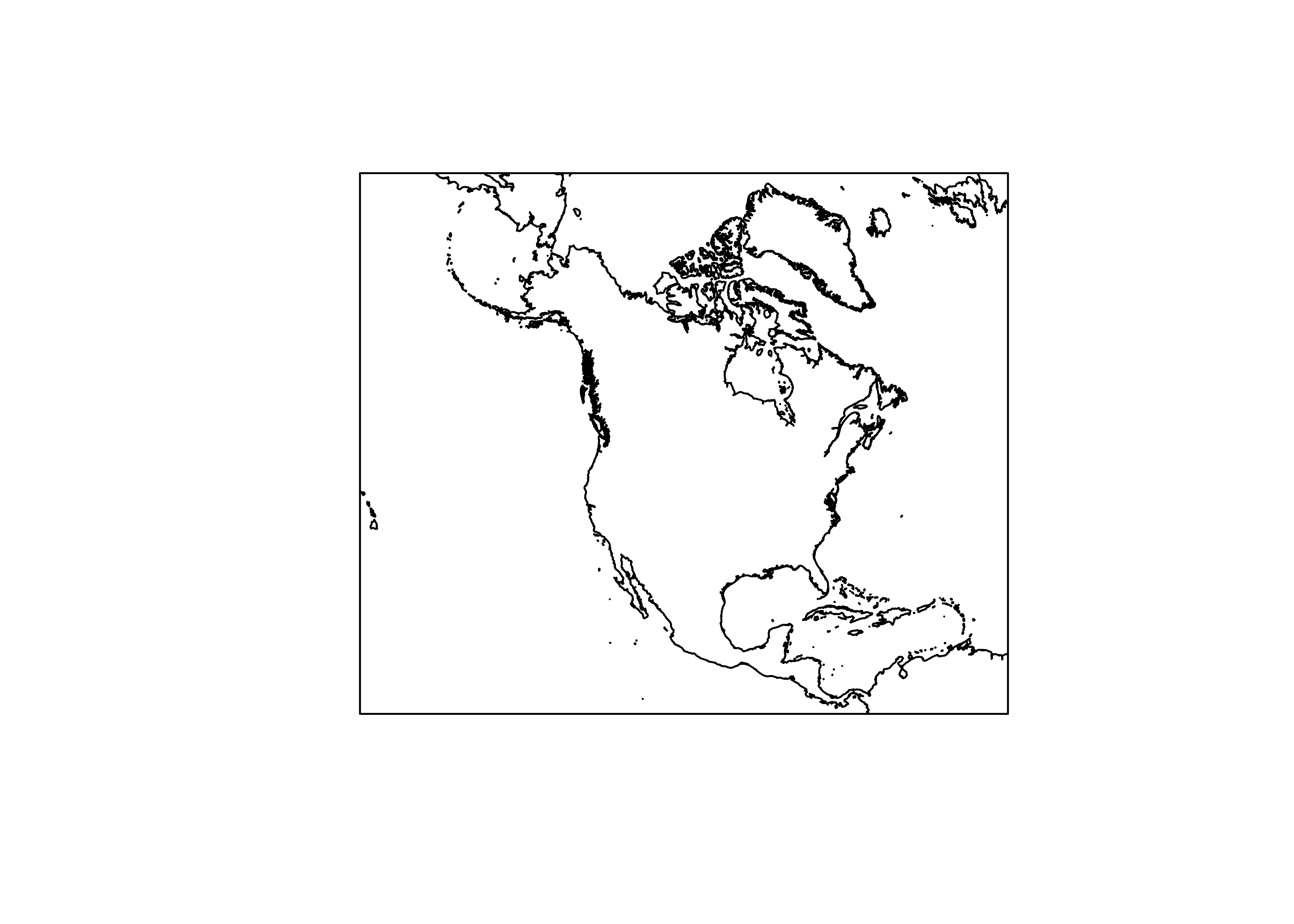
# trim the other projected objects
na10km_lakes_poly_proj <- st_intersection(lakes_poly_proj, na10km_bb)
na10km_lrglakes_poly_proj <- st_intersection(lrglakes_poly_proj, na10km_bb)
na10km_can_poly_proj <- st_intersection(can_poly_proj, na10km_bb)
na10km_us_poly_proj <- st_intersection(us_poly_proj, na10km_bb)
na10km_can_lines_proj <- st_intersection(can_lines_proj, na10km_bb)
na10km_us_lines_proj <- st_intersection(us_lines_proj, na10km_bb)
na10km_grat15_lines_proj <- st_intersection(grat15_lines_proj, na10km_bb)
na10km_admin0_poly_proj <- st_intersection(admin0_poly_proj, na10km_bb)
na10km_admin1_poly_proj <- st_intersection(admin1_poly_proj, na10km_bb)
Plot the projected shapefiles.
# plot the projected objects
plot(st_geometry(na10km_coast_lines_proj))
plot(st_geometry(na10km_can_lines_proj), col = "pink", add = TRUE)
plot(st_geometry(na10km_us_lines_proj), col = "lightblue", add = TRUE)
plot(st_geometry(na10km_lrglakes_poly_proj), col = "lightblue", bor = "blue", add=TRUE)
plot(st_geometry(na10km_admin0_poly_proj), bor = "gray70", add = TRUE)
plot(st_geometry(na10km_grat15_lines_proj), col = "gray70", add = TRUE)
plot(st_geometry(na10km_bb), border = "purple", add = TRUE)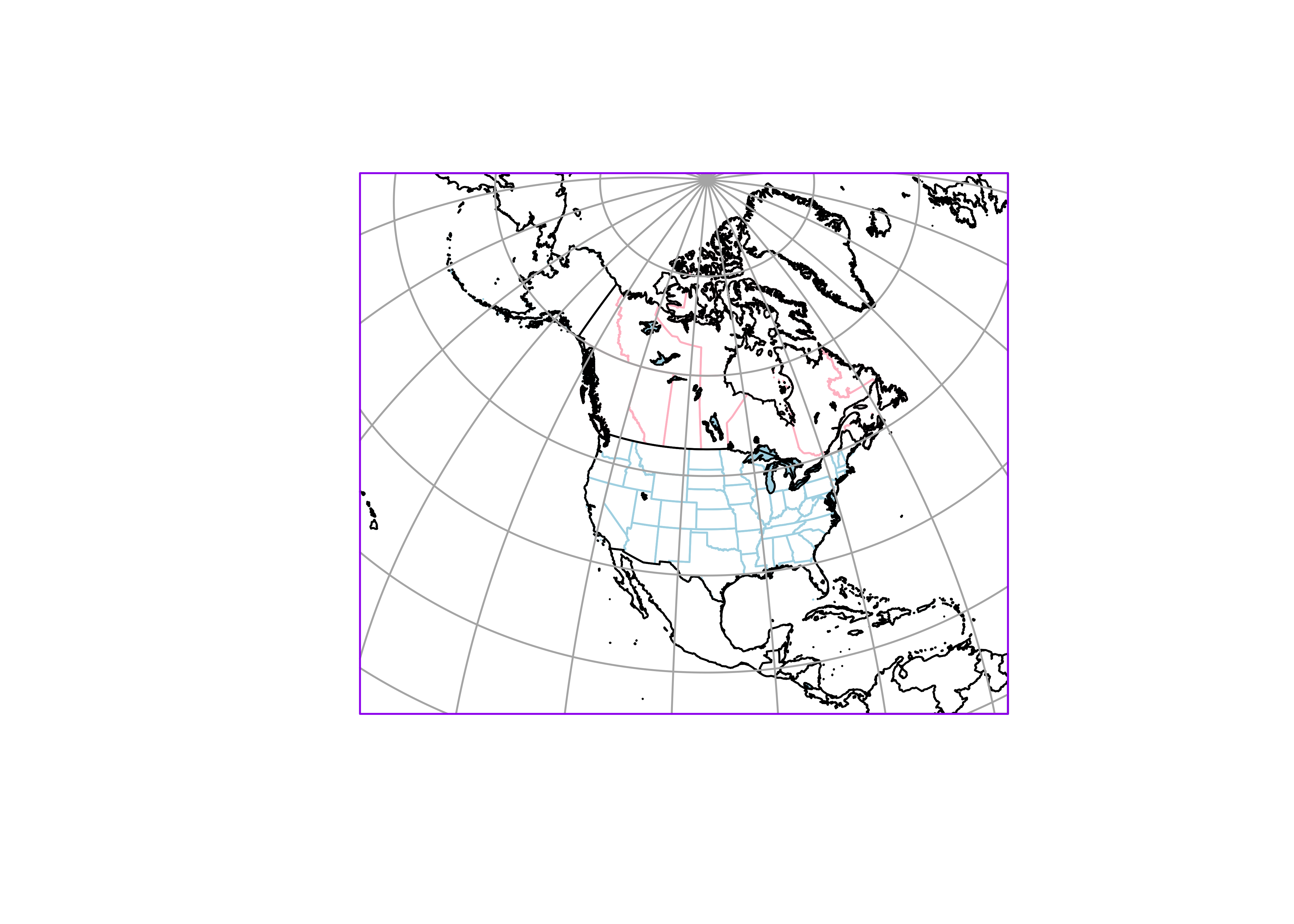
1.3 Write out the projected and trimmed shape files
Next, write out the projected shapefiles, first setting the output path.
# write out the various shapefiles
outpath <- "/Users/bartlein/Projects/RESS/data/RMaps/derived/na10km_10m/"
# coast lines
outshape <- na10km_coast_lines_proj
outfile <- "na10km_10m_coast_lines/"
outshapefile <- paste(outpath,outfile,sep="")
st_write(outshape, outshapefile, driver = "ESRI Shapefile", append = FALSE)## Deleting layer `na10km_10m_coast_lines' using driver `ESRI Shapefile'
## Writing layer `na10km_10m_coast_lines' to data source
## `/Users/bartlein/Projects/RESS/data/RMaps/derived/na10km_10m/na10km_10m_coast_lines/' using driver `ESRI Shapefile'
## Writing 1277 features with 2 fields and geometry type Unknown (any).It’s always good practice to test whether the shapefile has ideed been written out correctly. Read it back in and plot it.
## Reading layer `na10km_10m_coast_lines' from data source
##   `/Users/bartlein/Projects/RESS/data/RMaps/derived/na10km_10m/na10km_10m_coast_lines'
##   using driver `ESRI Shapefile'
## Simple feature collection with 1277 features and 2 fields
## Geometry type: MULTILINESTRING
## Dimension:     XY
## Bounding box:  xmin: -5770000 ymin: -4510000 xmax: 5e+06 ymax: 4480000
## Projected CRS: +proj=laea +lat_0=50 +lon_0=-100 +x_0=0 +y_0=0 +datum=WGS84 +units=m +no_defs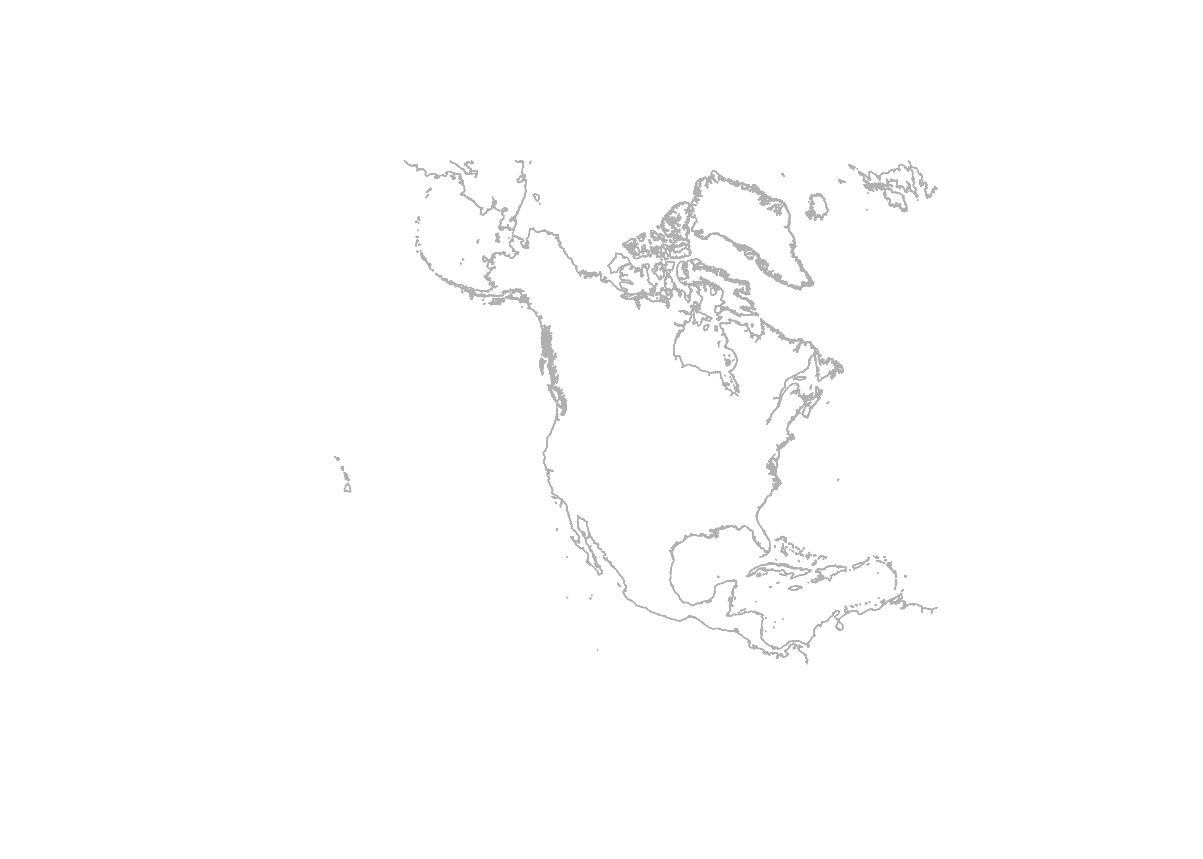
Write out the other shape files (output is suppressed):
# write out the various shapefiles
outshape <- na10km_bb
outfile <- "na10km_10m_bb/"
outshapefile <- paste(outpath,outfile,sep="")
st_write(outshape, outshapefile, driver = "ESRI Shapefile", append = FALSE)

# lakes poly
outshape <- na10km_lakes_poly_proj
outfile <- "na10km_10m_lakes_poly/"
outshapefile <- paste(outpath, outfile, sep="")
st_write(outshape, outshapefile, driver = "ESRI Shapefile", append = FALSE)

# lrglakes poly
outshape <- na10km_lrglakes_poly_proj
outfile <- "na10km_10m_lrglakes_poly"
outshapefile <- paste(outpath,outfile,sep="")
st_write(outshape, outshapefile, driver = "ESRI Shapefile", append = FALSE)

# can poly
outshape <- na10km_can_poly_proj
outfile <- "na10km_10m_can_poly/"
outshapefile <- paste(outpath,outfile,sep="")
st_write(outshape, outshapefile, driver = "ESRI Shapefile", append = FALSE)

# us poly
outshape <- na10km_us_poly_proj
outfile <- "na10km_10m_us_poly/"
outshapefile <- paste(outpath,outfile,sep="")
st_write(outshape, outshapefile, driver = "ESRI Shapefile", append = FALSE)

# can lines
outshape <- na10km_can_lines_proj
outfile <- "na10km_10m_can_lines/"
outshapefile <- paste(outpath,outfile,sep="")
st_write(outshape, outshapefile, driver = "ESRI Shapefile", append = FALSE)

# us lines
outshape <- na10km_us_lines_proj
outfile <- "na10km_10m_us_lines/"
outshapefile <- paste(outpath,outfile,sep="")
st_write(outshape, outshapefile, driver = "ESRI Shapefile", append = FALSE)

# admin0 poly
outshape <- na10km_admin0_poly_proj
outfile <- "na10km_10m_admin0_poly/"
outshapefile <- paste(outpath,outfile,sep="")
st_write(outshape, outshapefile, driver = "ESRI Shapefile", append = FALSE)

# admin1 poly
outshape <- na10km_admin1_poly_proj
outfile <- "na10km_10m_admin1_poly/"
outshapefile <- paste(outpath,outfile,sep="")
st_write(outshape, outshapefile, driver = "ESRI Shapefile", append = FALSE)2 Map of North American shaded relief
2.1 PlotØ the projected and trimmed shapefiles
If necessary (i.e. if starting here), read the projected shapefiles:
# plot the basemap (note different order than before)
plot(st_geometry(na10km_bb), border = "black", col = "aliceblue")
plot(st_geometry(na10km_grat15_lines_proj), col = "gray70", add = TRUE)
plot(st_geometry(na10km_admin0_poly_proj), col = "white",  border = "gray", add = TRUE)
plot(st_geometry(na10km_can_lines_proj), col = "gray", add = TRUE)
plot(st_geometry(na10km_us_lines_proj), col = "gray", add = TRUE)
plot(st_geometry(na10km_lrglakes_poly_proj), col = "aliceblue", border = "black", lwd = 0.5, add = TRUE)
plot(st_geometry(na10km_coast_lines_proj), col = "black", lwd = 0.5, add = TRUE)
plot(st_geometry(na10km_bb), boder = "black", add = TRUE)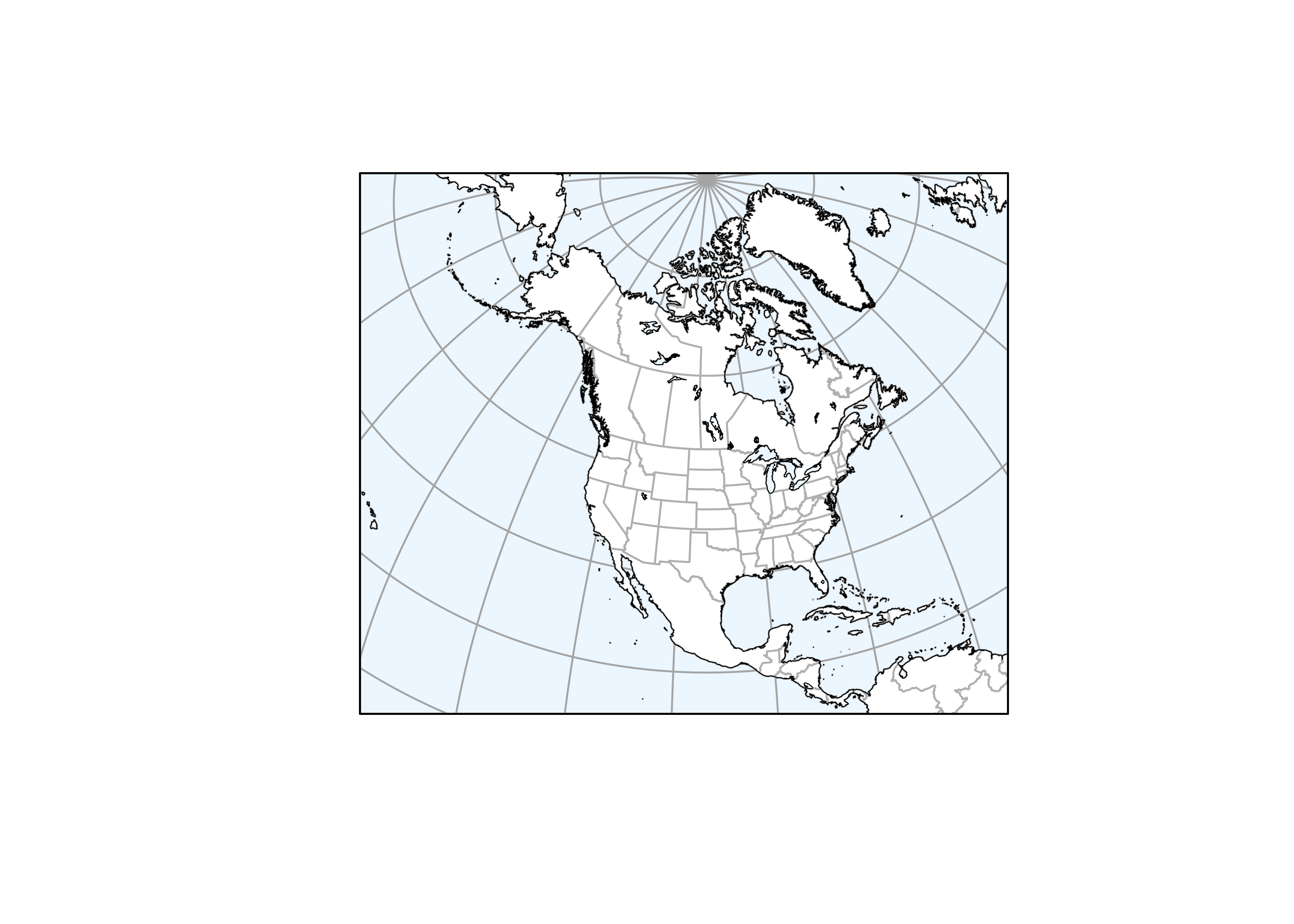
2.2 Read a shaded relief file
Read a pre-computed shaded relief file. This could also be crearted
by reading the na10km_v2 grid-point elevations and using the
shade function from the terra package. Note
that in this file, the coordinates are in km, and so they must be
multiplied by 1000.
# get 10km shade values
datapath <- "/Users/bartlein/Projects/RESS/data/csv_files/"
datafile <- "na10km_shade.csv"
shade <- read.csv(paste(datapath,datafile,sep=""))
str(shade)
## 'data.frame': 282017 obs. of 5 variables:
## $ x : num -5770 -5760 -5720 -5720 -5720 -5720 -5710 -5710 -5710 -5710 ...
## $ y : num -820 -820 -860 -850 -840 -830 -870 -860 -850 -840 ...
## $ shade: num 0.691 0.691 0.31 0.334 0.559 ...
## $ lat : num 21.8 21.9 21.9 22 22 ...
## $ lon : num -160 -160 -160 -160 -160 ...## x y shade lat lon
## 1 -5770000 -820000 0.691208 21.83661 -160.1851
## 2 -5760000 -820000 0.691208 21.90175 -160.1023
## 3 -5720000 -860000 0.310095 21.90119 -159.5651
## 4 -5720000 -850000 0.333957 21.96637 -159.6163
## 5 -5720000 -840000 0.559432 22.03148 -159.6676
## 6 -5720000 -830000 0.956591 22.09651 -159.7191Convert the dataframe to a POINTS sf object
# convert to POINTS
shade_pixels <- st_as_sf(shade, coords = c("x", "y"), crs = na_crs)
shade_pixels
## Simple feature collection with 282017 features and 3 fields
## Geometry type: POINT
## Dimension: XY
## Bounding box: xmin: -5770000 ymin: -4510000 xmax: 5e+06 ymax: 4480000
## Projected CRS: +proj=laea +lon_0=-100 +lat_0=50 +x_0=0 +y_0=0 +ellps=WGS84 +datum=WGS84 +units=m +no_defs
## First 10 features:
## shade lat lon geometry
## 1 0.691208 21.83661 -160.1851 POINT (-5770000 -820000)
## 2 0.691208 21.90175 -160.1023 POINT (-5760000 -820000)
## 3 0.310095 21.90119 -159.5651 POINT (-5720000 -860000)
## 4 0.333957 21.96637 -159.6163 POINT (-5720000 -850000)
## 5 0.559432 22.03148 -159.6676 POINT (-5720000 -840000)
## 6 0.956591 22.09651 -159.7191 POINT (-5720000 -830000)
## 7 0.481249 21.90038 -159.4309 POINT (-5710000 -870000)
## 8 0.081382 21.96570 -159.4820 POINT (-5710000 -860000)
## 9 0.123170 22.03093 -159.5332 POINT (-5710000 -850000)
## 10 0.850642 22.09609 -159.5846 POINT (-5710000 -840000)Read some predetermined (gray-scale) colors for the shading.
# read hillshade color numbers
colorfile <- "shade40_clr.csv"
shade_rgb <- read.csv(paste(datapath, colorfile, sep=""))
shade_clr <- rgb(shade_rgb)
Set the (gray-scale) color numbers for each pixel:
2.3 Make the map
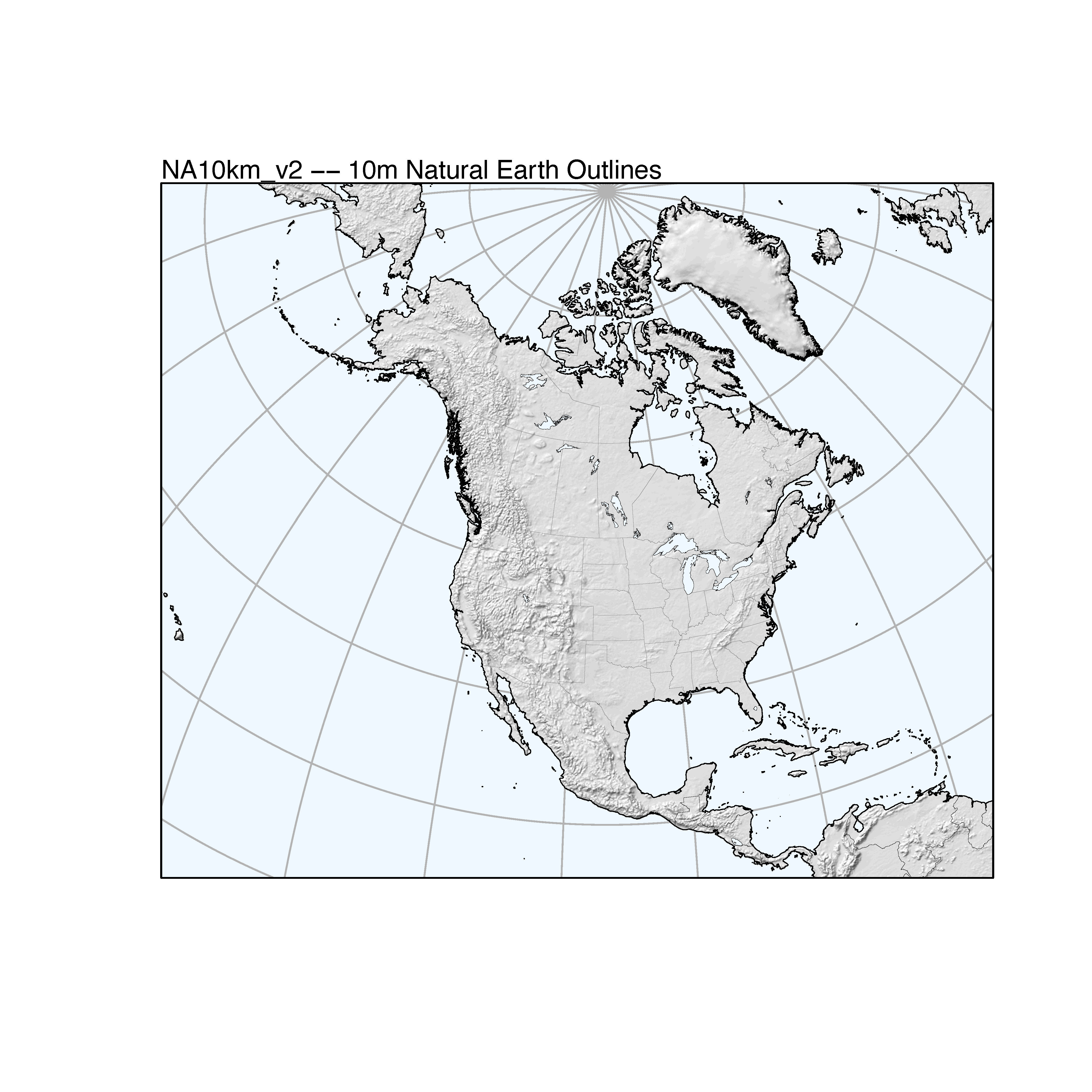
Plot the shaded-relief colors and the various shape files. The
location of the text string was determined by plotting an initial
version of the map, and using the locator() function. The
cex=0.09 argument in plotting shade_pixels was
determined by trial and error. Redirect the output to a .pdf file.
pdf(file = "na_shade01b.pdf")
plot(st_geometry(na10km_bb), border = "black", col = "aliceblue")
plot(st_geometry(na10km_grat15_lines_proj), col = "gray70", add = TRUE)
plot(st_geometry(shade_pixels), pch=15, cex=0.09, col=shade_colnum, add = TRUE)
plot(st_geometry(na10km_admin0_poly_proj), lwd=0.2, bor="gray50", add=TRUE)
plot(st_geometry(na10km_can_lines_proj), lwd=0.2, col="gray50", add=TRUE)
plot(st_geometry(na10km_us_lines_proj), lwd=0.2, col="gray50", add=TRUE)
plot(st_geometry(na10km_lrglakes_poly_proj), lwd=0.2, bor="black", col="aliceblue", add=TRUE)
plot(st_geometry(na10km_coast_lines_proj), lwd=0.5, add=TRUE)
text(-5770000, 4620000, pos=c(4), offset=0.0, cex=1.0, "NA10km_v2 -- 10m Natural Earth Outlines")
plot(st_geometry(na10km_bb), add=TRUE)
dev.off()
The resulting plot will look like this:
3 Mapping the western U.S. precipitation-ratio data
A final example describes mapping the western U.S. precipitation data
via the {ggplot2} package, as seen in the [Using
R: Examples]. Here, the basemap will be extracted from the
{maps} package (and later compared with the Natural Earth
shapefiles basemap versions).
3.1 Get and project basemap outlies
Get oulines for the western states. the map() function
retrieves the outlines from the maps() package database,
and st_as_sf(), converts those to and (unprojected)
MULTIPOLYGONS sf object:
library(maps)

# get outlines of western states from {maps} package
wus_sf <- st_as_sf(map("state", regions=c("washington", "oregon", "california", "idaho", "nevada",
    "montana", "utah", "arizona", "wyoming", "colorado", "new mexico", "north dakota", "south dakota",
    "nebraska", "kansas", "oklahoma", "texas"), plot = FALSE, fill = TRUE))
head(wus_sf); tail(wus_sf)
## Simple feature collection with 6 features and 1 field
## Geometry type: MULTIPOLYGON
## Dimension: XY
## Bounding box: xmin: -124.3834 ymin: 31.34652 xmax: -94.58387 ymax: 49.00508
## Geodetic CRS: +proj=longlat +ellps=clrk66 +no_defs +type=crs
## ID geom
## arizona arizona MULTIPOLYGON (((-114.6374 3...
## california california MULTIPOLYGON (((-120.006 42...
## colorado colorado MULTIPOLYGON (((-102.0552 4...
## idaho idaho MULTIPOLYGON (((-117.0266 4...
## kansas kansas MULTIPOLYGON (((-94.63544 3...
## montana montana MULTIPOLYGON (((-104.0491 4...## Simple feature collection with 6 features and 1 field
## Geometry type: MULTIPOLYGON
## Dimension: XY
## Bounding box: xmin: -124.6813 ymin: 25.9378 xmax: -93.53536 ymax: 49.00508
## Geodetic CRS: +proj=longlat +ellps=clrk66 +no_defs +type=crs
## ID geom
## oregon oregon MULTIPOLYGON (((-116.9292 4...
## south dakota south dakota MULTIPOLYGON (((-96.43452 4...
## texas texas MULTIPOLYGON (((-94.49792 3...
## utah utah MULTIPOLYGON (((-114.0472 4...
## washington washington MULTIPOLYGON (((-123.0198 4...
## wyoming wyoming MULTIPOLYGON (((-109.0511 4...## [1] "sf" "data.frame"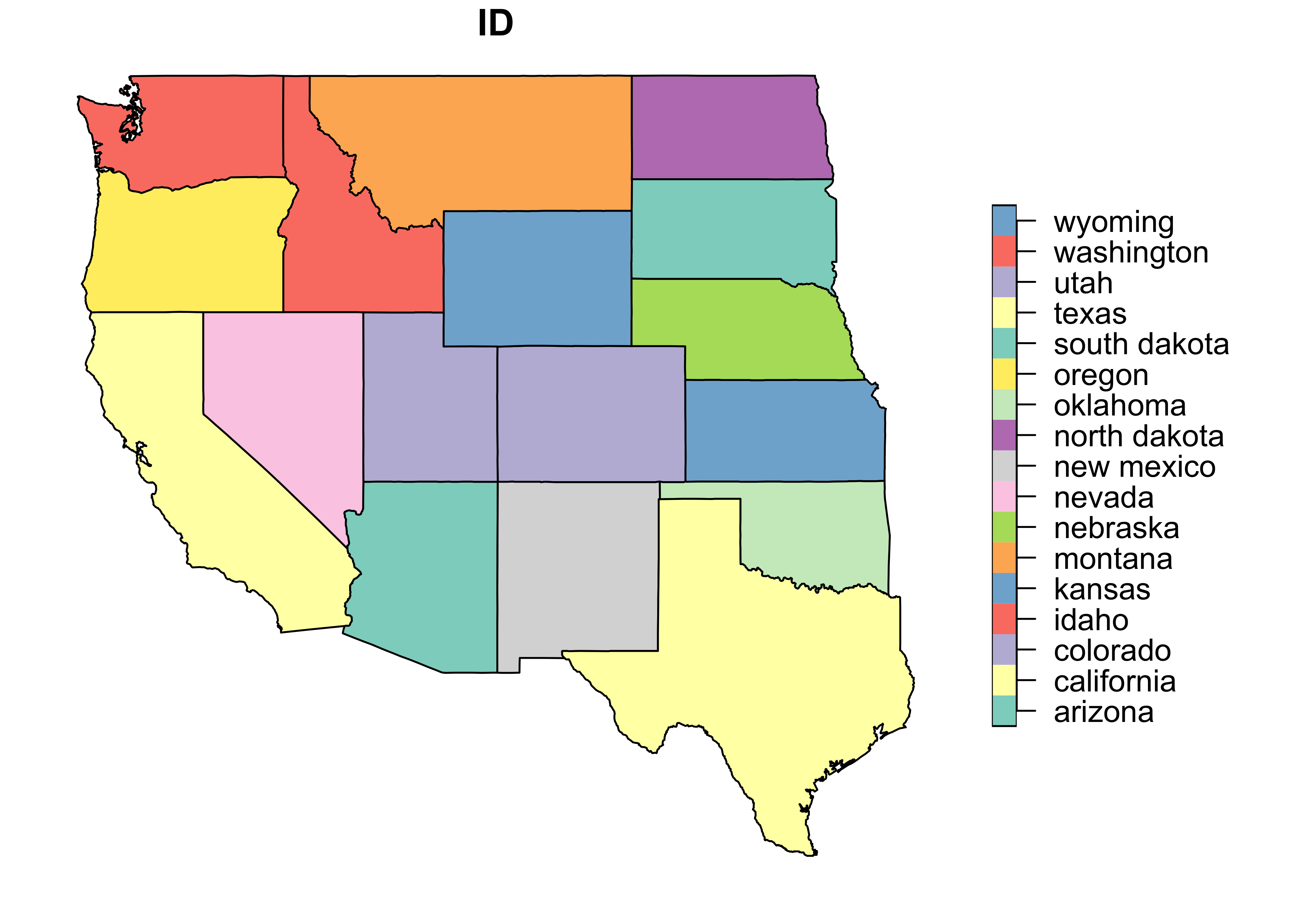
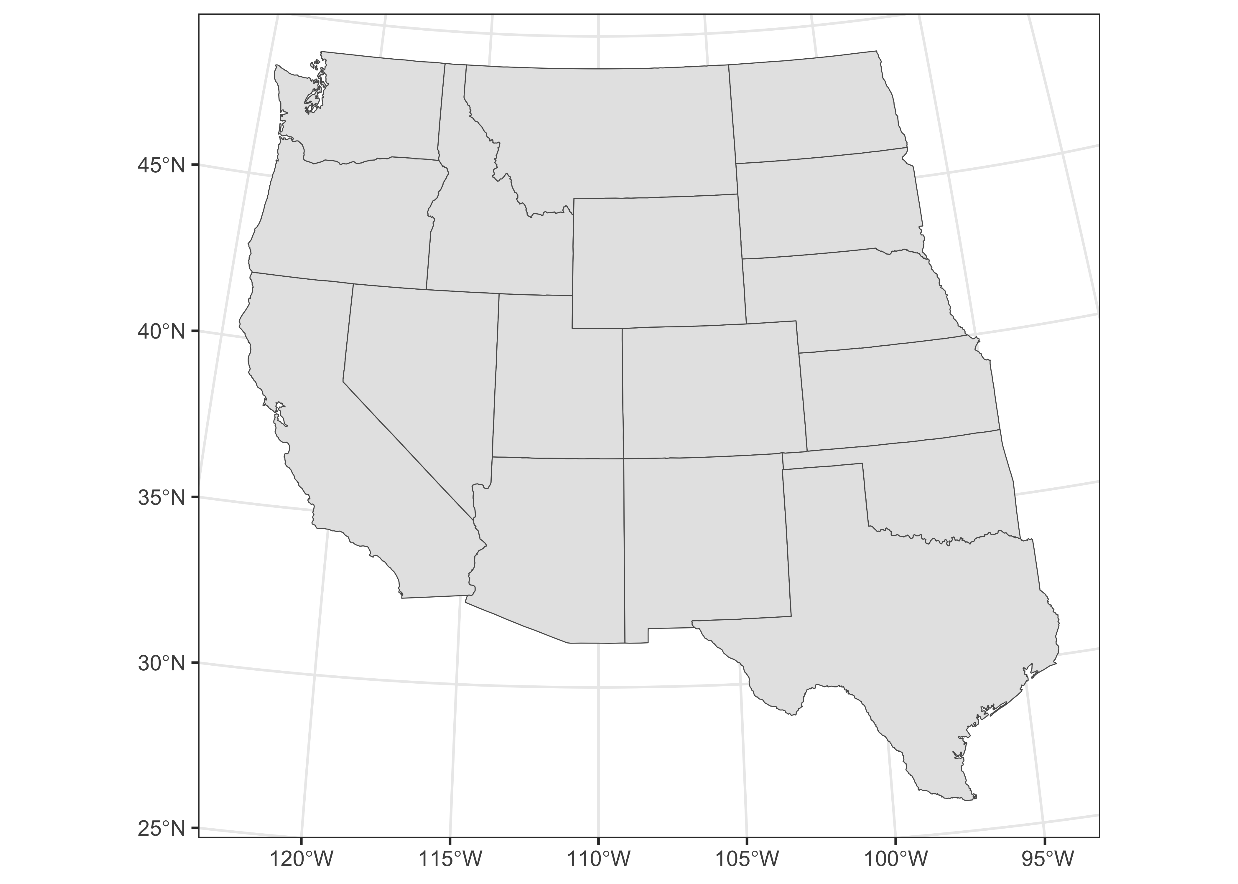
Here’s a quick ggplot2 map of the outlines:
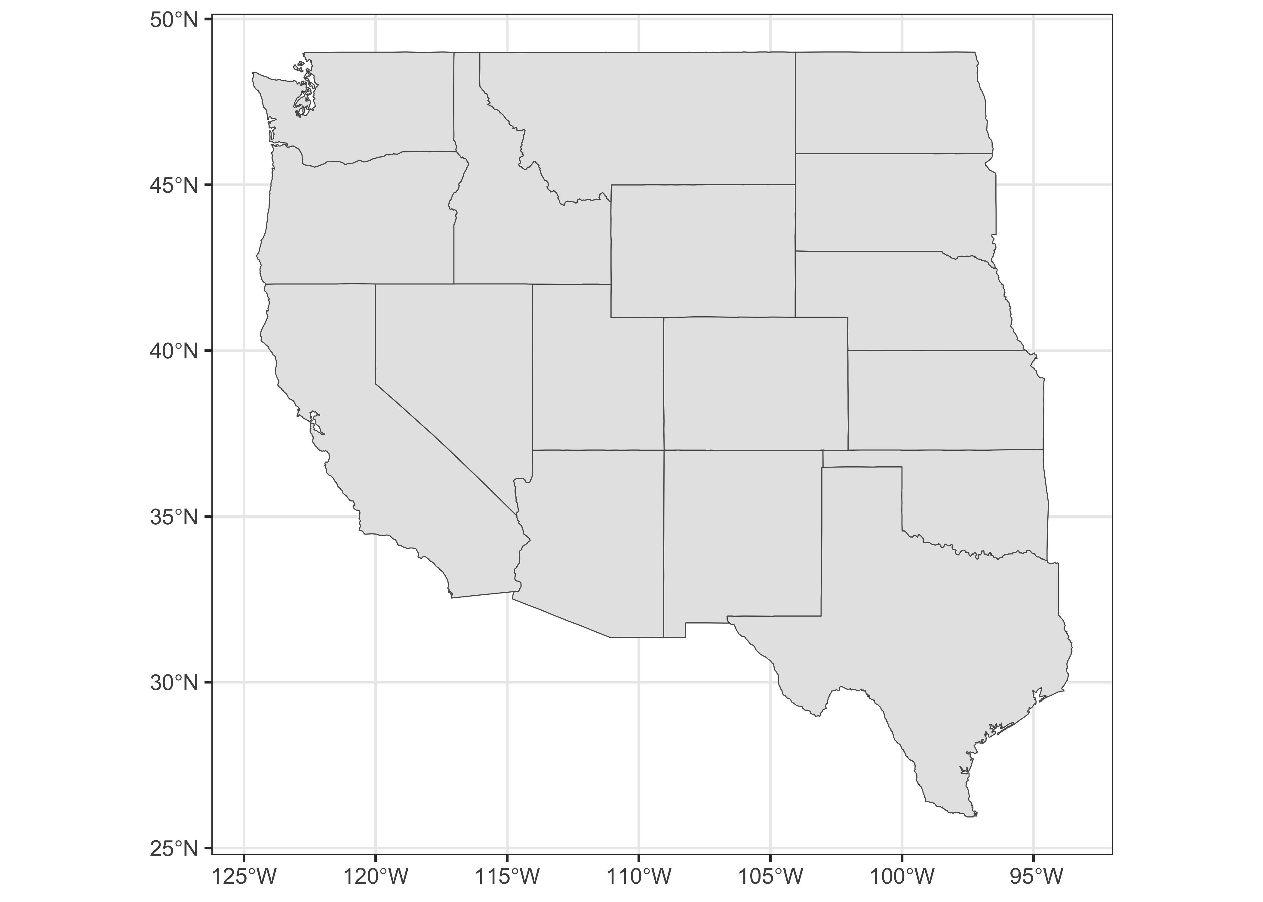
Project the outlines and a graticule (extracted from the
wus_sf object using st_graticule()):
# projection
laea = st_crs("+proj=laea +lat_0=30 +lon_0=-110") # Lambert Azimuthal Equal Area
wus_sf_proj = st_transform(wus_sf, laea)
plot(st_geometry(wus_sf_proj), axes = TRUE)
plot(st_geometry(st_graticule(wus_sf_proj)), axes = TRUE, add = TRUE)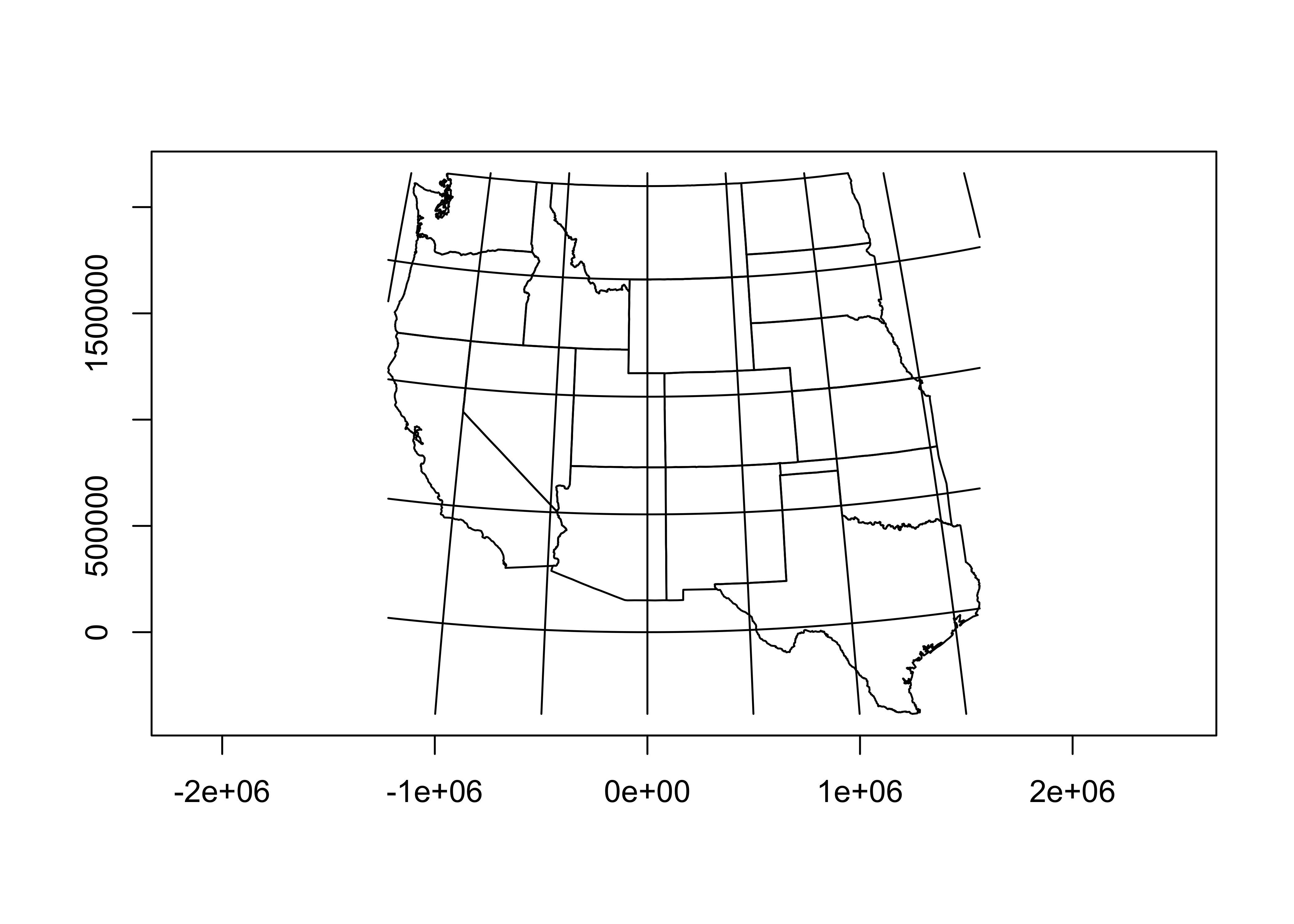
Note the coordinates are now in meters.
Here’s a ggplot2 version:
Get two other outlines from the maps database, one for
all of North America, and the other for the U.S.”
# get two other outlines
na_sf <- st_as_sf(map("world", regions=c("usa", "canada", "mexico"), plot = FALSE, fill = TRUE))
conus_sf <- st_as_sf(map("state", plot = FALSE, fill = TRUE))
Because sf objects are basically dataframes, they can be
manipulated using some of the common R functions, like
rbind (row bind). Combine the na_sf and
conus_sf objects, and plot them out:
## Simple feature collection with 6 features and 1 field
## Geometry type: MULTIPOLYGON
## Dimension:     XY
## Bounding box:  xmin: -178.1945 ymin: 14.54541 xmax: 179.78 ymax: 83.11611
## Geodetic CRS:  +proj=longlat +ellps=clrk66 +no_defs +type=crs
##                ID                           geom
## Canada     Canada MULTIPOLYGON (((-59.7876 43...
## Mexico     Mexico MULTIPOLYGON (((-91.68369 1...
## USA           USA MULTIPOLYGON (((-155.5813 1...
## alabama   alabama MULTIPOLYGON (((-87.46201 3...
## arizona   arizona MULTIPOLYGON (((-114.6374 3...
## arkansas arkansas MULTIPOLYGON (((-94.05103 3...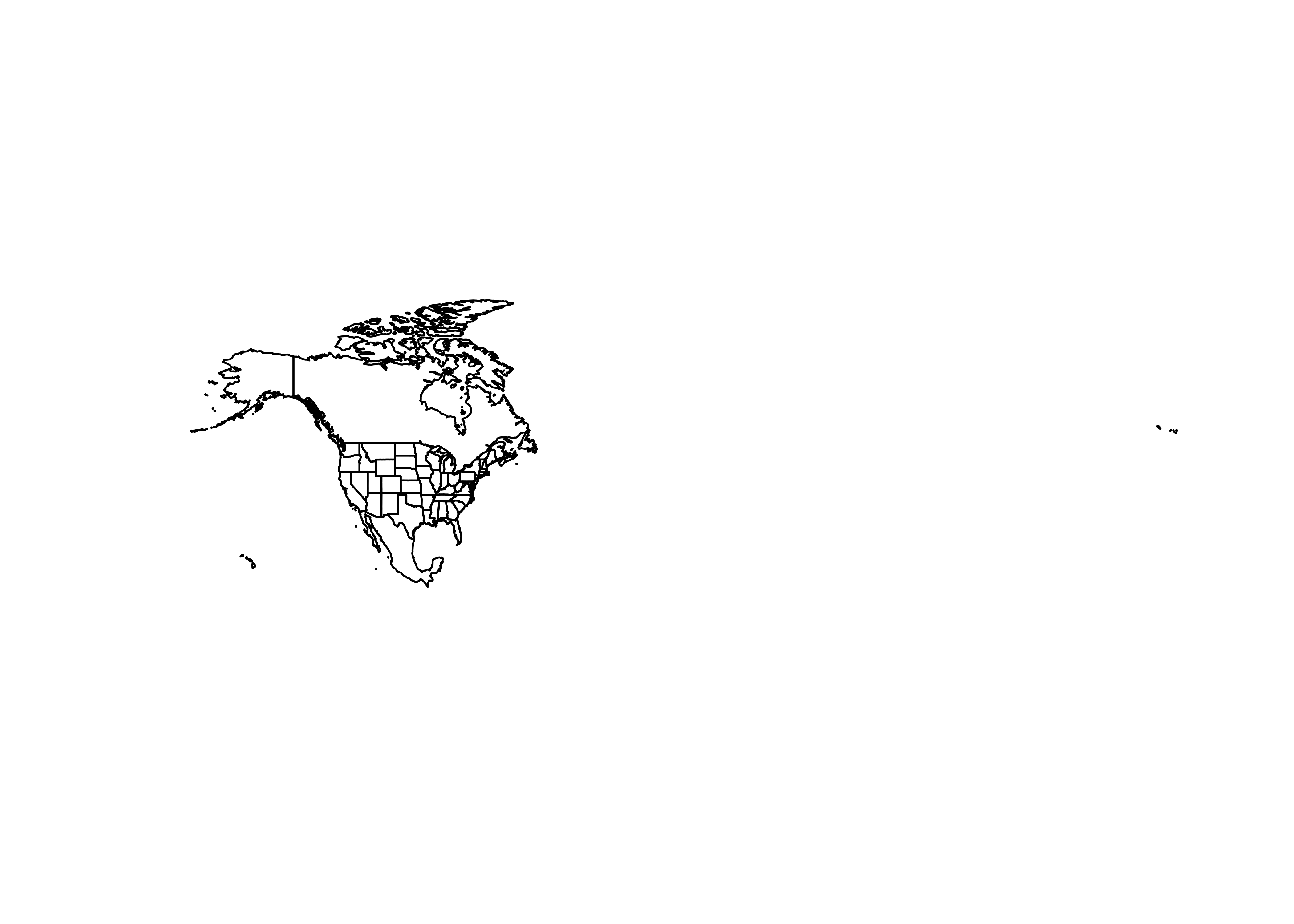
Note that the map is slightly strange–the Aleutians cross the dateline (180W), so the map wraps around.
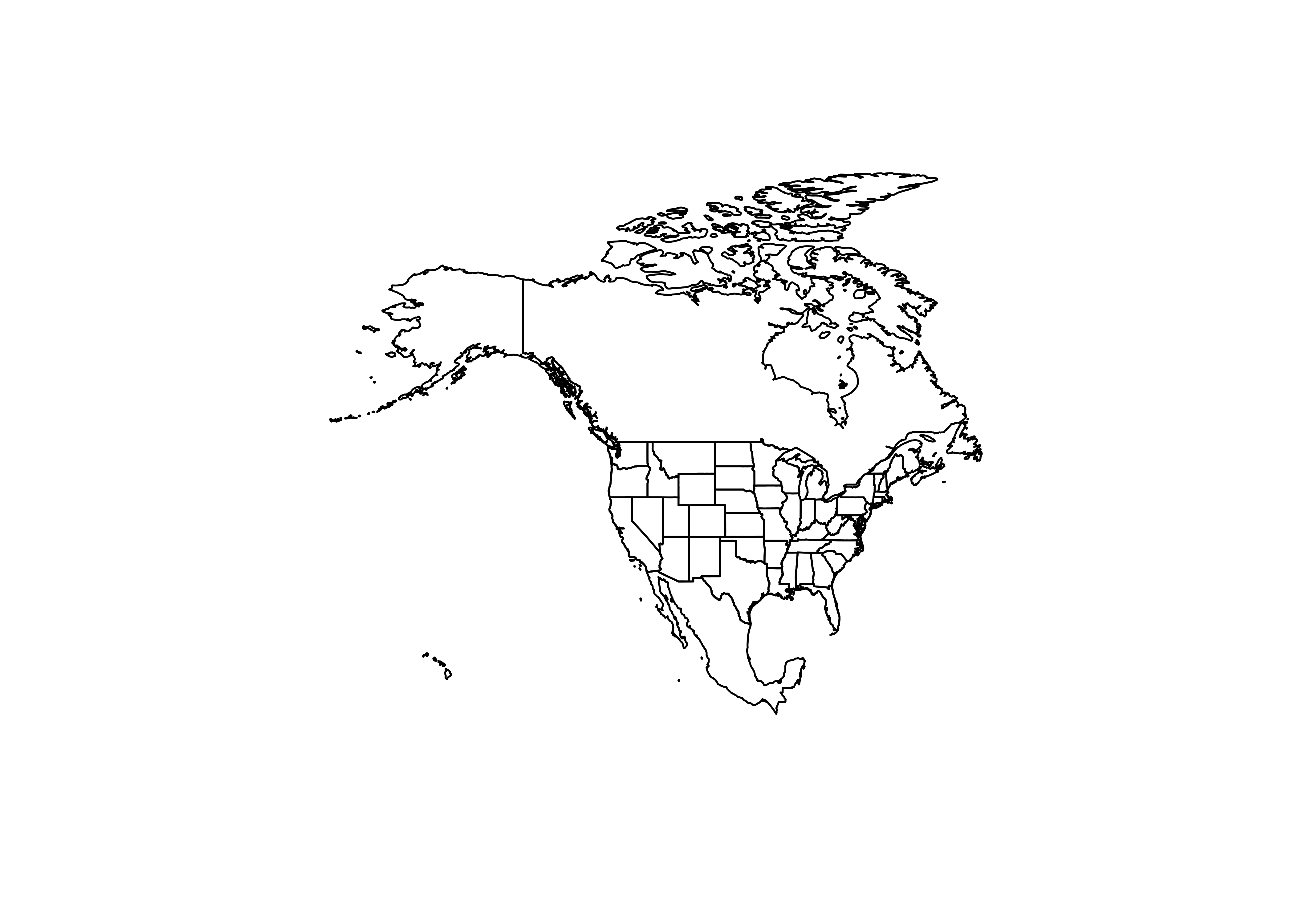
Project the additional outlines:
# project the other outlines
na_sf_proj = st_transform(na_sf, laea)
conus_sf_proj = st_transform(conus_sf, laea)
na2_sf_proj = st_transform(na2_sf, laea)
# plot everthing so far
plot(st_geometry(na_sf_proj), col = "red", axes = TRUE)
plot(st_geometry(wus_sf_proj), axes = TRUE, add = TRUE)
plot(st_geometry(st_graticule(wus_sf_proj)), add = TRUE)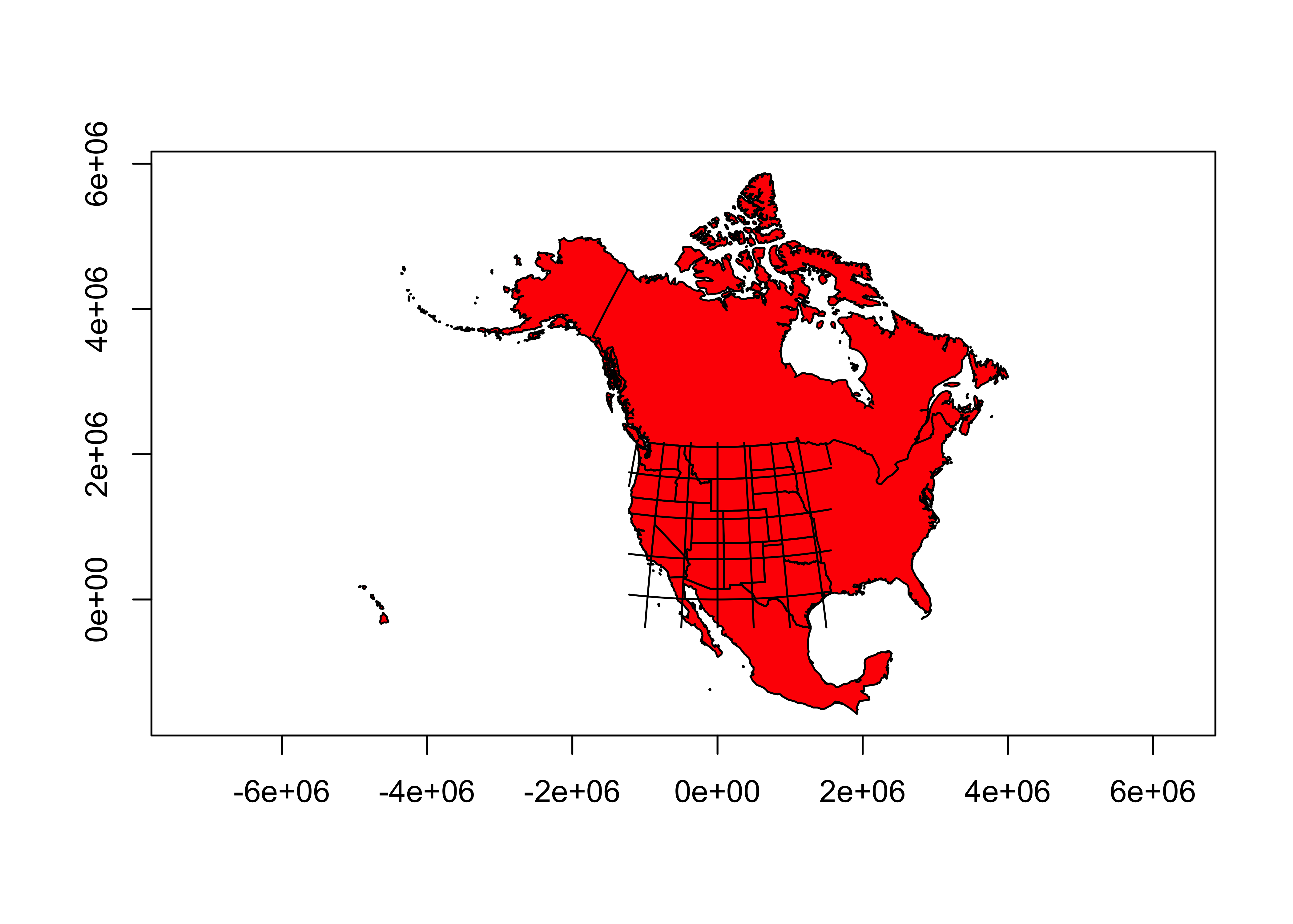
3.2 Get and project the pratio data
# pratios
csv_path <- "/Users/bartlein/Projects/RESS/data/csv_files/"
csv_file <- "wus_pratio.csv"
wus_pratio <- read.csv(paste(csv_path, csv_file, sep = ""))
Make an sf object:
# make an sf object
wus_pratio_sf <- st_as_sf(wus_pratio, coords = c("lon", "lat"))
plot(st_geometry(wus_pratio_sf), pch=16, cex = 0.5)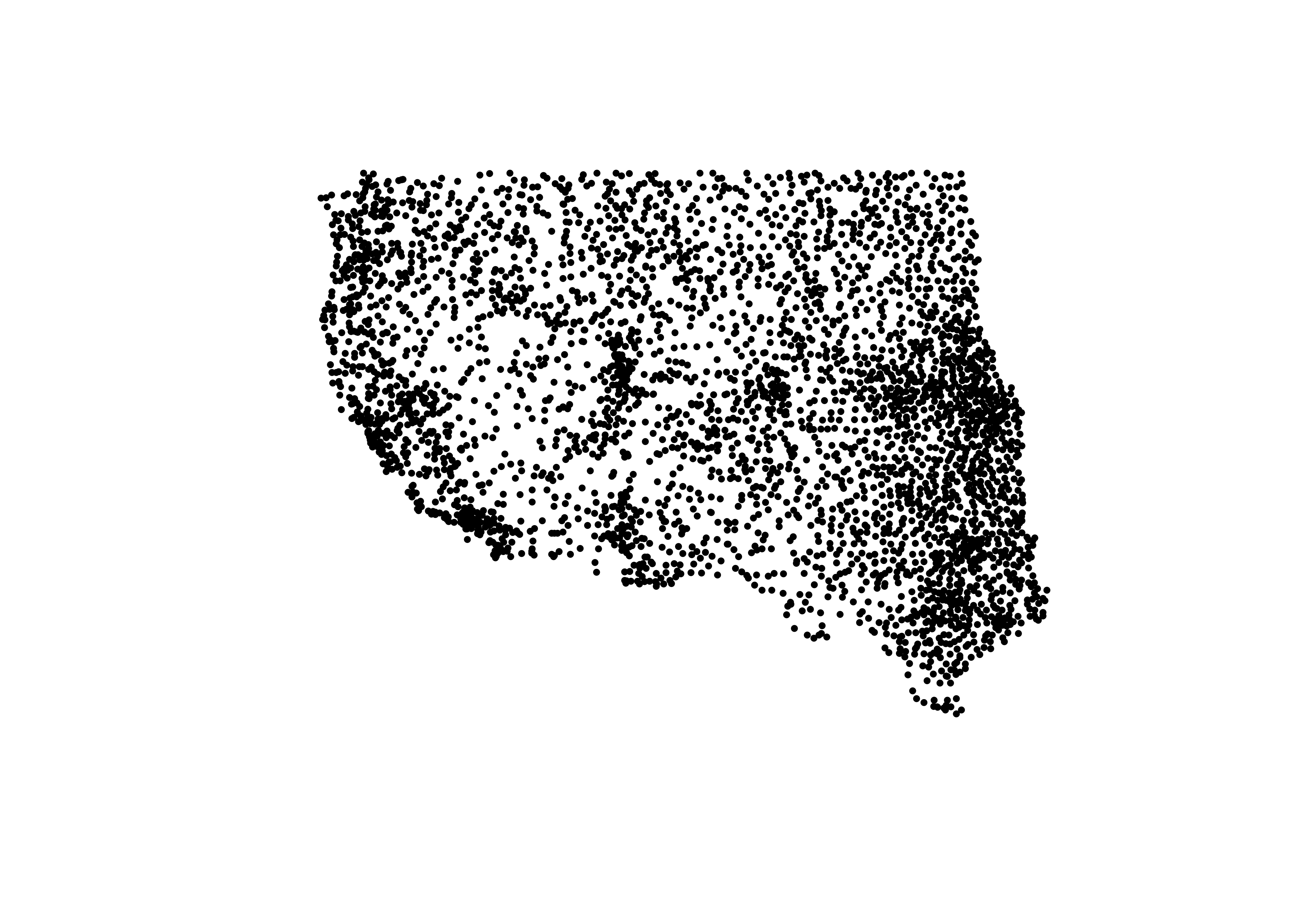
Recode the the pjulpann ratio to a factor:
# recode pjulpjan to a factor
library(classInt)
wus_pratio$pjulpjan <- wus_pratio$pjulpann/wus_pratio$pjanpann  # pann values cancel out
cutpts <- c(0.0, .100, .200, .500, .800, 1.0, 1.25, 2.0, 5.0, 10.0, 9999.0)
pjulpjan_factor <- factor(findInterval(wus_pratio$pjulpjan, cutpts))
head(cbind(wus_pratio$pjulpjan, pjulpjan_factor, cutpts[pjulpjan_factor]))
## pjulpjan_factor
## [1,] 0.43465046 3 0.2
## [2,] 1.15409836 6 1.0
## [3,] 0.05609915 1 0.0
## [4,] 0.26222597 3 0.2
## [5,] 0.05042017 1 0.0
## [6,] 0.14257556 2 0.1Here’s an (unprojected) map of the precipitation ratio:
## ggplot2 map of pjulpjan
ggplot() +
  geom_sf(data = wus_sf, fill=NA) +
  scale_color_brewer(type = "div", palette = "PRGn", aesthetics = "color", direction = 1,
                    labels = c("0.0 - 0.1", "0.1 - 0.2", "0.2 - 0.5", "0.5 - 0.8", "0.8 - 1.0",
                                "1.0 - 1.25", "1.25 - 2.0", "2.0 - 5.0", "5.0 - 10.0", "> 10.0"),
                    name = "Jul:Jan Ppt. Ratio") +
  labs(title = "Precipitation Seasonality", x = "Longitude", y = "Latitude") +
  geom_point(aes(wus_pratio$lon, wus_pratio$lat, color = pjulpjan_factor), size = 1.5 ) +
  theme_bw()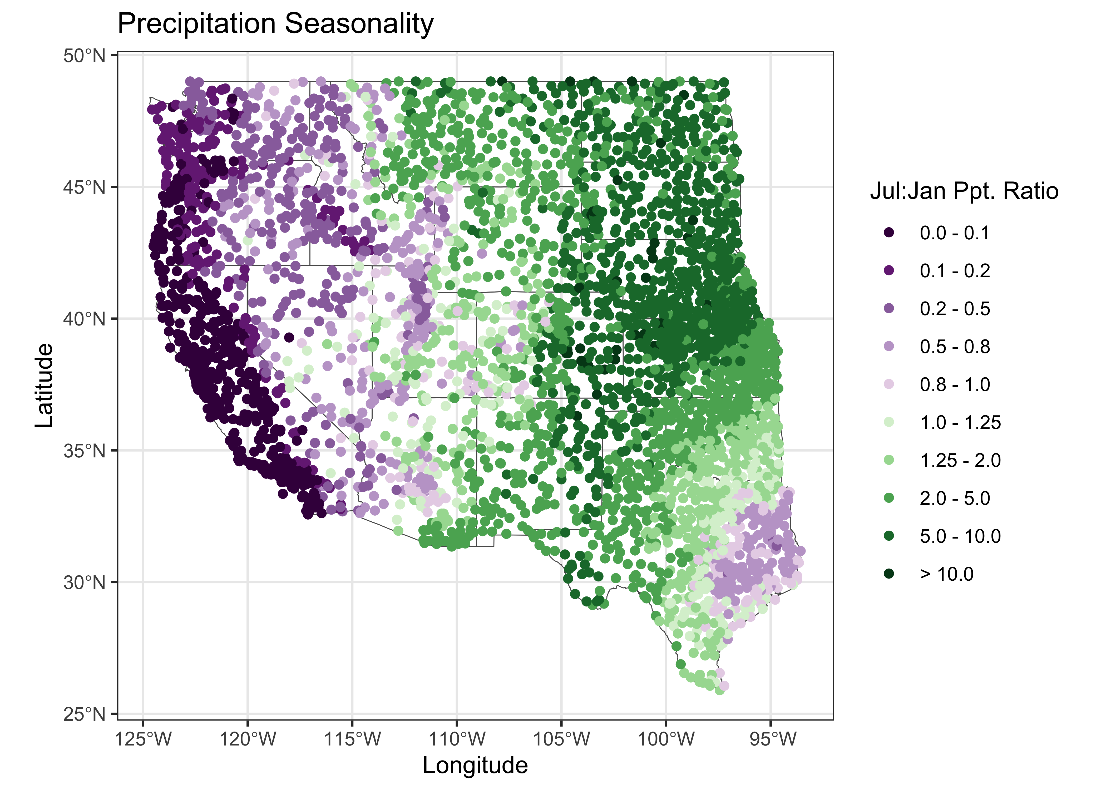
Project the precipitation ratio point
# projection
st_crs(wus_pratio_sf) <- st_crs("+proj=longlat")
laea = st_crs("+proj=laea +lat_0=30 +lon_0=-110") # Lambert equal area
wus_pratio_sf_proj = st_transform(wus_pratio_sf, laea)
Plot the projected points:
# plot the projected points
plot(st_geometry(wus_pratio_sf_proj), pch=16, cex=0.5, axes = TRUE)
plot(st_geometry(st_graticule(wus_pratio_sf_proj)), axes = TRUE, add = TRUE)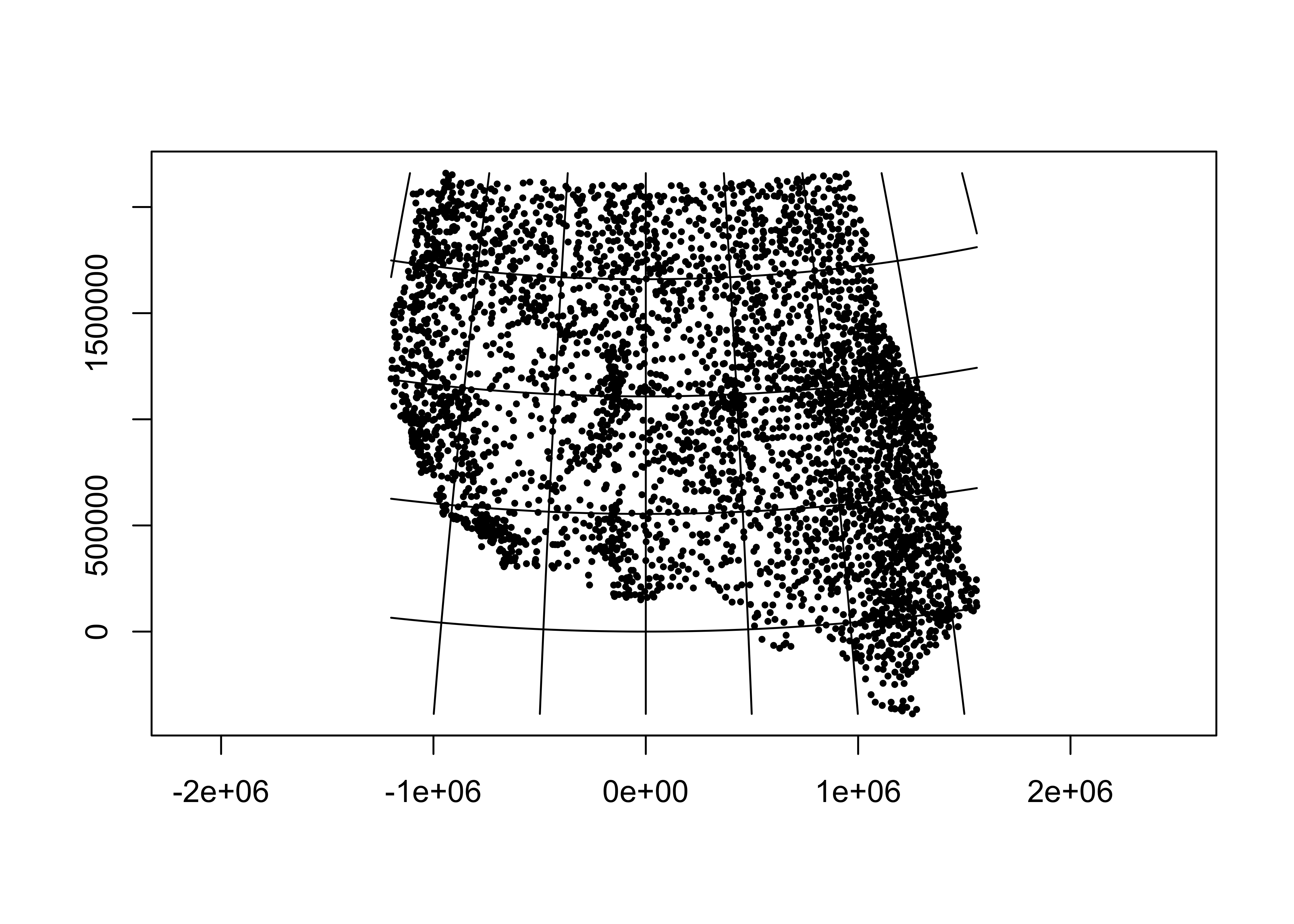 Plot everything
# ggplot2 map of pjulpman projected
ggplot() +
  geom_sf(data = na2_sf_proj, fill=NA, color="gray") +
  geom_sf(data = wus_sf_proj, fill=NA) +
  geom_sf(data = wus_pratio_sf_proj, aes(color = pjulpjan_factor), size = 1.0 ) +
  scale_color_brewer(type = "div", palette = "PRGn", aesthetics = "color", direction = 1,
              labels = c("0.0 - 0.1", "0.1 - 0.2", "0.2 - 0.5", "0.5 - 0.8", "0.8 - 1.0",
                        "1.0 - 1.25", "1.25 - 2.0", "2.0 - 5.0", "5.0 - 10.0", "> 10.0"),
              name = "Jul:Jan Ppt. Ratio") +
              labs(x = "Longitude", y = "Latitude") +
  guides(color = guide_legend(override.aes = list(size = 3))) +
  coord_sf(crs = st_crs(wus_sf_proj), xlim = c(-1400000, 1500000), ylim = c(-400000, 2150000)) +
  labs(title = "Precipitation Seasonality", x = "Longitude", y = "Latitude") +
  theme_bw()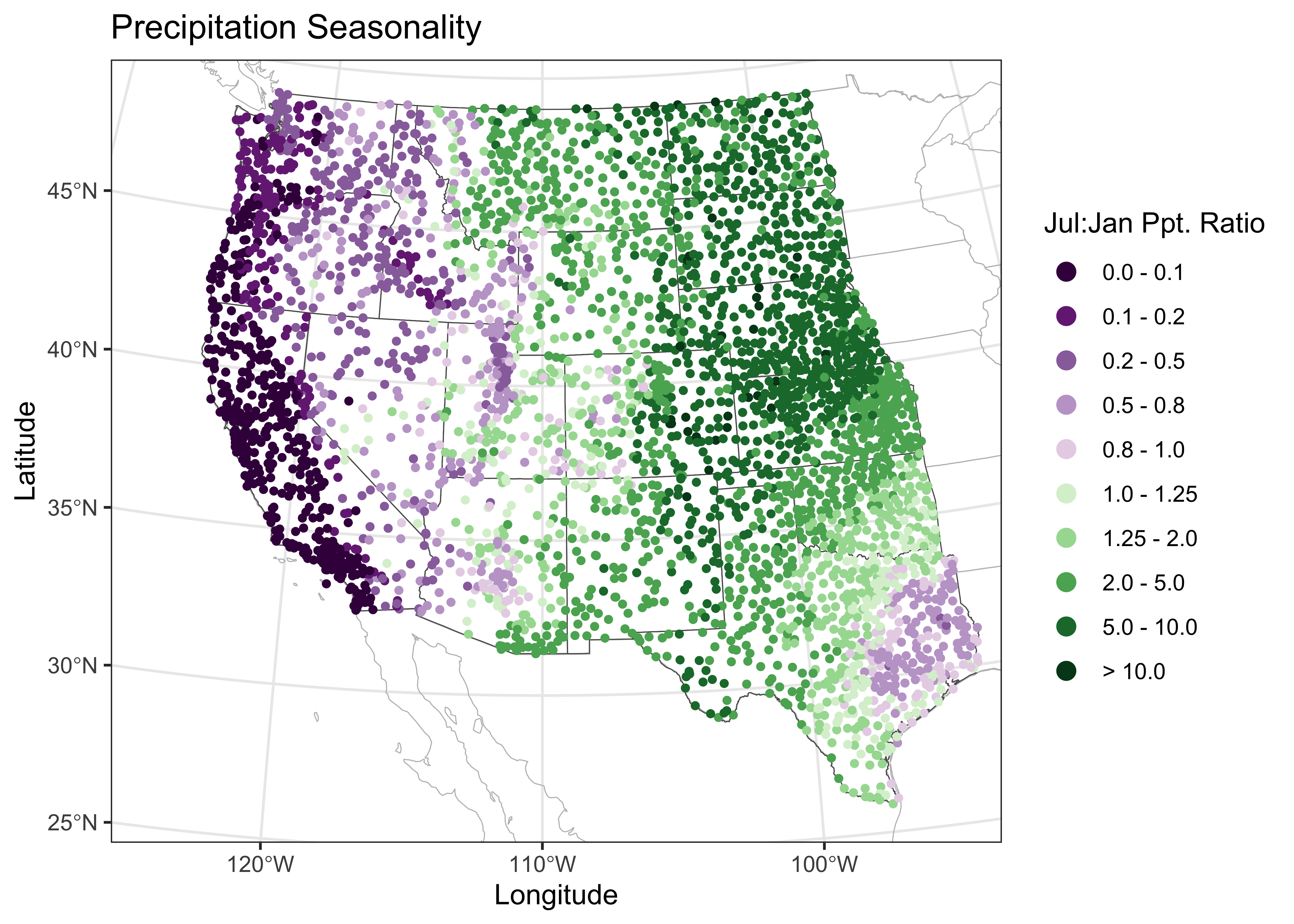
The guides() function expands the size (diameter) of the
legend key (size = 3) leaving the points at their original
size.
4 Compare shapefiles
While we have two differnet sources of shapefiles in the environment
(if all of the code chunks have been run), it would be useful to compare
them. Copy the following code into a script window. Then run the script
a line at a time. The first line will just set up a plotting region.
Then the next three lines will plot in turn the Natural Earth outlines
of the coastlines and the U.S. and Canada. Note that the outlines
overlay one another exactly (there’s no black visible). Then
run the next two lines, one at a time to plot {maps}
package outlines. Notice what happens along the coast, and in particular
around Vancouver Is. and the Puget Sound. The fact that the Natural
Earth outlines are still visible, as are the separate
{maps} package outlines implies that the various shape
files are not coregisterd.
# outlines
# from the Natural Earth shapefile collection
plot(NULL, NULL, xlim = c(-130.0, -110), ylim = c(40.0, 50.0),
xlab = "Longitude", ylab = "Latitude")
plot(st_geometry(coast_lines_sf), border = "black", add = TRUE)
plot(st_geometry(can_poly_sf), border = "purple", add = TRUE)
plot(st_geometry(us_poly_sf), border = "magenta", add = TRUE)
# from the maps package
plot(st_geometry(na_sf), border = "red", add = TRUE)
plot(st_geometry(wus_sf), border = "blue", add = TRUE)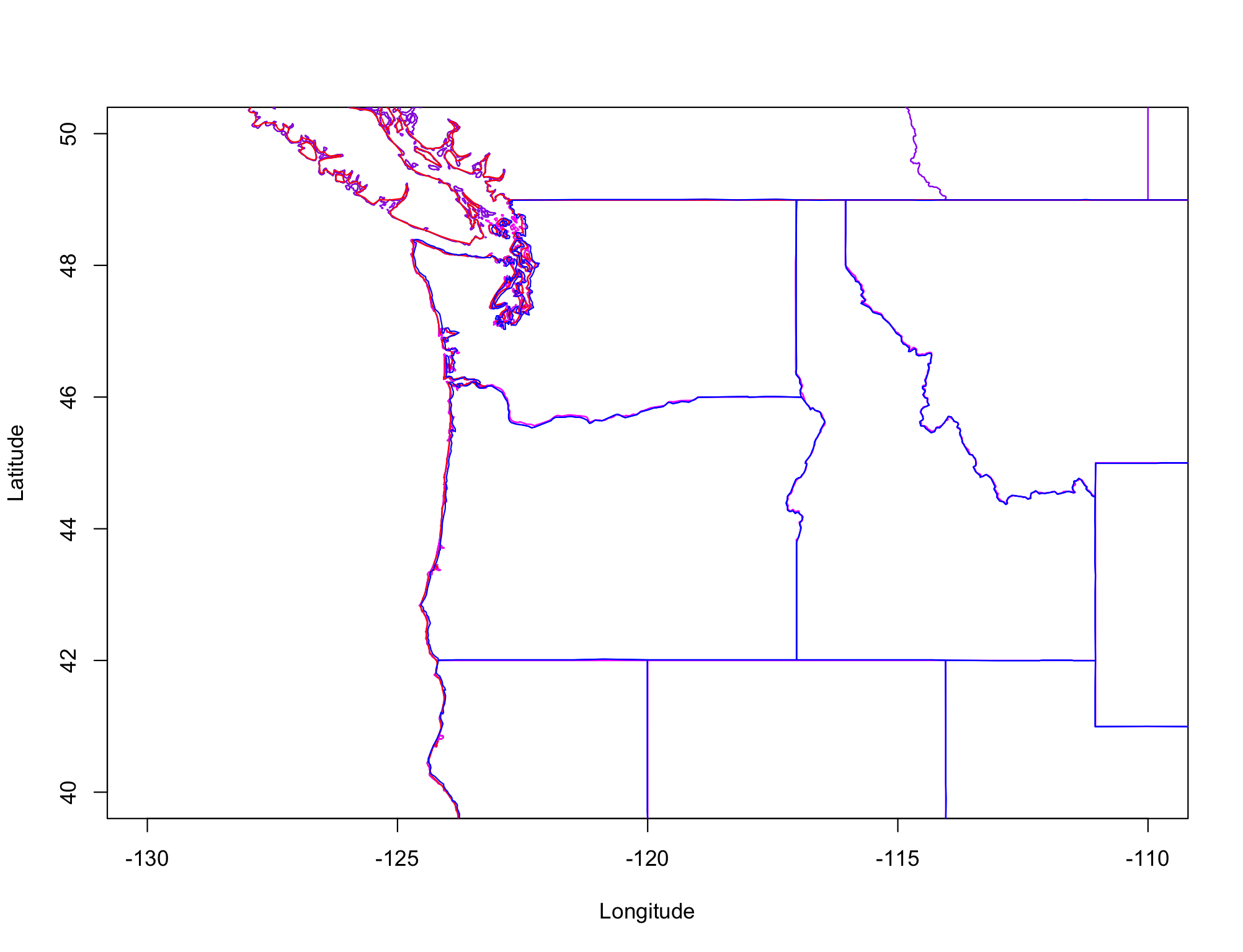 Do the same thing for the following
code, which plots the vertices along the MULTILINESTRINGS.
Do the same thing for the following
code, which plots the vertices along the MULTILINESTRINGS.
# verticies (points)
# from the Natural Earth shapefile collection
plot(NULL, NULL, xlim = c(-130.0, -110), ylim = c(40.0, 50.0),
     xlab = "Longitude", ylab = "Latitude")
points(st_coordinates(coast_lines_sf), col = "black", pch = 16, cex = 0.4)
points(st_coordinates(can_poly_sf), col = "purple", pch = 16, cex = 0.5)
points(st_coordinates(us_poly_sf), col = "magenta", pch = 16, cex = 0.5)

# from the maps package
points(st_coordinates(na_sf), col = "red", pch = 16, cex = 0.5)
points(st_coordinates(wus_sf), col = "blue", pch = 16, cex = 0.5)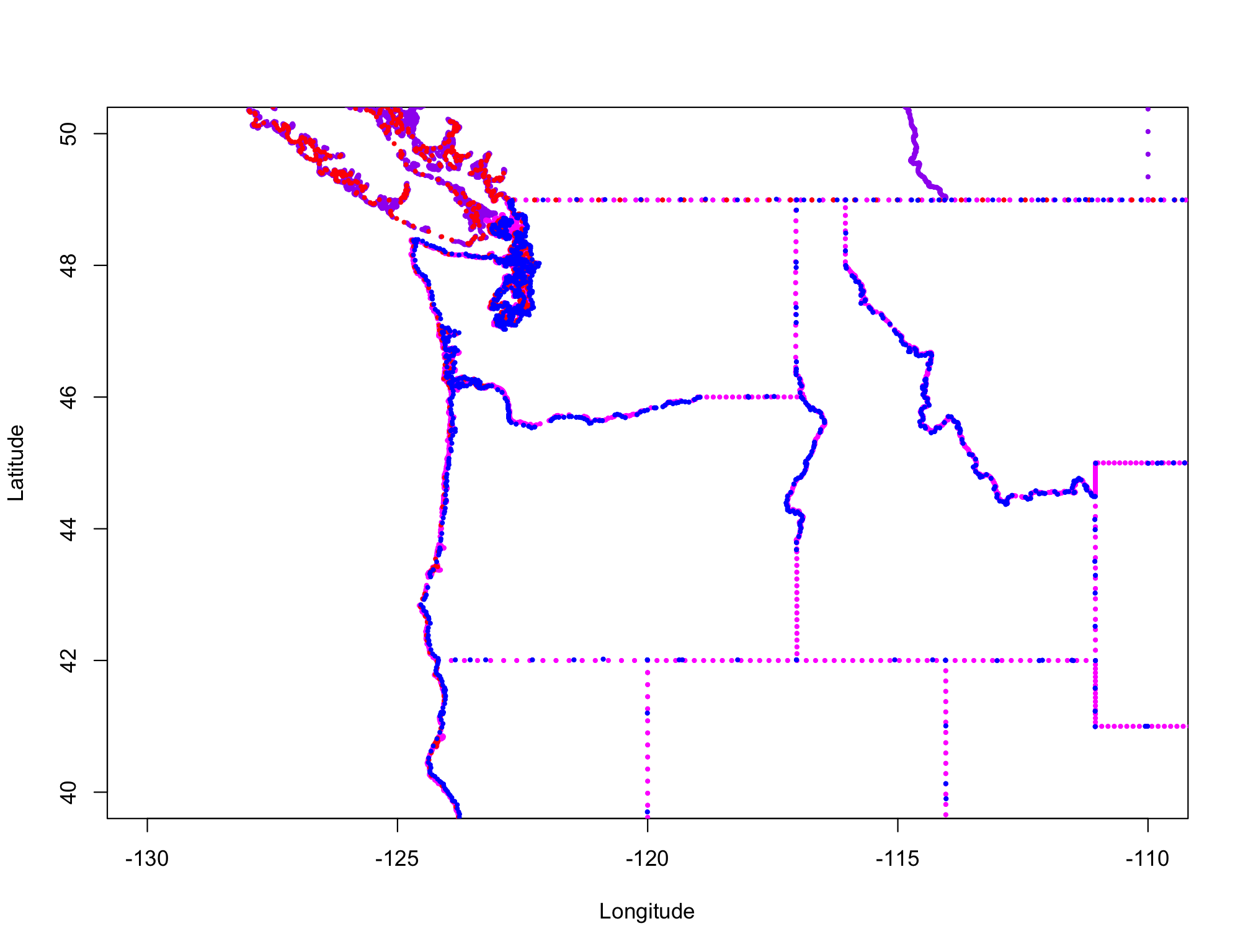
Ugh!