Data wrangling and matrix algebra

NOTE: This page has been revised for Winter 2021, but may undergo further edits.

1 Introduction

This lecture focuses on two topics that underlie R’s facility for reading and analyzing data: 1) the facility for reading and transforming (i.e. tidying) data that may not initially be in standard “rectangular data set” form, and 2) the manipulation of arrays, vectors and matrices of data “under the hood” in the execution of various data-analysis routines. The first topic, which also has been termed “data wrangling” is also an element of the concept of “reproducible research” which aims at documenting the analysis steps and results with sufficient detail that they could be reproduced by others.

Often, data are available in a format that might be efficient for one reason or another, but may not be in the tidy arrangement of variables in columns and observations or cases in rows. Although it is possible to coerce such data into the standard rectangular or “data frame” layout, perhaps by using Excel or by simple cutting and pasting in a text editor, that approach may not be reproducible, in the sense of having a body of code that can be rerun on the same or similar data sets. By doing the reorganization or reshaping within R, and documenting the analysis using R Markdown, the specific steps involved in the reshaping of the data can be reproduced using that documented code. The tidying of data is supported by several packages that are elements of what Hadley Wickham (see the readings below) calls the “tidyverse” – these packages include readr (for reading various kind of text data), and dplyr and tidyr for manipulation.

Here are links to the RStudio cheat sheets for readr, dplyr, and tidyr:

• readr and tidyr [https://github.com/rstudio/cheatsheets/raw/master/data-import.pdf]
• dplyr [https://github.com/rstudio/cheatsheets/raw/master/data-transformation.pdf]

The second topic matrix algebra can be thought of as an efficient way of documenting the specific manipulations of or operations on data that are used to develop specific data-analysis results, by representing those operations in a very efficient and elegant manner. It is also the case, however, that matrix algebra is used in an analytical (as well as representational) sense to develop the specific statistics and their properties that are produced during an analysis. This will be illustrated later for regression and multivariate analysis.

2 Data wrangling

2.1 Example data

A simple example of data wrangling, or the reshaping of non-rectangular data set into a rectangular one, can be illustrated using a small sample of monthly climate data for Eugene. These data are not currently part of the geog495.RData workspace file, but can be dowloaded here:

• EugeneClim-short.csv – Three years (2013-2015) of monthly climate data for Eugene;
• EugeneClim-short-alt-tvars.csv – Temperature data for those three years in an alternative format that is not tidy (i.e. columns are months (or observations) and rows are variables); and
• EugeneClim-short-alt-pvars.csv – Precipitation data, also in an alternative format.

The full data set can be downloaded from here: EugeneClim.csv

2.1.1 Variables

The variables in the data set include:

• TMAX – Monthly/Annual Maximum Temperature. Average of daily maximum temperature
• TMIN – Monthly/Annual Minimum Temperature. Average of daily minimum temperature
• TAVG – Average Monthly/Annual Temperature. Computed by adding the unrounded monthly/annual maximum and minimum temperatures and dividing by 2.
• EMXT – Extreme maximum temperature for month/year. Highest daily maximum temperature for the month/year.
• EMNT – Extreme minimum temperature for month/year. Lowest daily minimum
• HTDD - Heating Degree Days. Computed when daily average temperature is less than 65 degrees Fahrenheit/18.3 degrees Celsius. HDD = 65(F)/18.3(C) – mean daily temperature. Each day is summed to produce a monthly/annual total.
• CLDD - Cooling Degree Days. Computed when daily average temperature is more than 65 degrees Fahrenheit/18.3 degrees Celsius. CDD = mean daily temperature - 65 degrees Fahrenheit/18.3 degrees Celsius. Each day is summed to produce a monthly/annual total.
• PRCP – Total Monthly/Annual Precipitation. Given in inches or millimeters depending on user specification.
• EMXP – Highest daily total of precipitation in the month/year.
• DP01 – Number of days with >= 0.01 inch/0.254 millimeter in the month/year.
• DP05 – Number of days with >= 0.5 inch/12.7 millimeters in the month/year.
• DP10 – Number of days with >= 1.00 inch/25.4 millimeters in the month/year.
• SNOW – Total Monthly/Annual Snowfall.
• EMSD – Highest daily snow depth in the month/year
• AWND – Monthly/Annual Average Wind Speed.

(Variable names in the files are in lower case.)

2.2 Read the data

The “short” (3-year) data set can be read in the conventional way, as a data.frame object:

# read the .csv file conventionally
csv_file <- "/Users/bartlein/Documents/geog495/data/csv/EugeneClim-short.csv"
eugclim_df <- read.csv(csv_file) 

Notice the name of the function that was used to read the .csv file: read.csv().

The class() and str() functions can be used to figure out the kind and format of the data:

class(eugclim_df)

## [1] "data.frame"

str(eugclim_df)

## 'data.frame':    36 obs. of  18 variables:
##  $ year: int  2013 2013 2013 2013 2013 2013 2013 2013 2013 2013 ...
##  $ mon : int  1 2 3 4 5 6 7 8 9 10 ...
##  $ yrmn: num  2013 2013 2013 2013 2013 ...
##  $ tmax: num  5.7 10.2 14.5 17 21.1 25 30.6 28.6 23.1 16.5 ...
##  $ tmin: num  -0.4 2.3 3 4.6 6.9 9.8 10.8 12.7 11.9 3.9 ...
##  $ tavg: num  2.6 6.3 8.7 10.8 14 17.4 20.7 20.7 17.5 10.2 ...
##  $ emxt: num  13.3 13.9 22.2 25.6 30 35.6 35.6 35 32.2 25.6 ...
##  $ emnt: num  -6.7 -2.8 -2.2 -0.5 1.1 4.4 6.1 7.8 5 -2.1 ...
##  $ htdd: num  487 338 298 226 137 ...
##  $ cldd: num  0 0 0 0 2.5 25.3 77.7 79.2 33.1 0 ...
##  $ prcp: num  34.5 41 54.2 36.8 51.7 ...
##  $ emxp: num  6.4 11.2 12.7 11.9 13 18.3 0 3.8 48.3 8.4 ...
##  $ dp01: int  11 14 12 10 13 7 0 4 15 6 ...
##  $ dp05: int  0 0 1 0 1 1 0 0 6 0 ...
##  $ dp10: int  0 0 0 0 0 0 0 0 1 0 ...
##  $ snow: int  NA NA NA NA NA 0 0 0 NA NA ...
##  $ emsd: int  NA NA NA 0 0 0 0 0 0 0 ...
##  $ awnd: num  1.9 2.6 2.2 2.7 3.1 2.5 3.4 2.5 3.2 1.7 ...

eugclim_df

##    year mon     yrmn tmax tmin tavg emxt  emnt  htdd  cldd  prcp emxp dp01 dp05 dp10 snow emsd awnd
## 1  2013   1 2013.000  5.7 -0.4  2.6 13.3  -6.7 486.9   0.0  34.5  6.4   11    0    0   NA   NA  1.9
## 2  2013   2 2013.083 10.2  2.3  6.3 13.9  -2.8 337.9   0.0  41.0 11.2   14    0    0   NA   NA  2.6
## 3  2013   3 2013.167 14.5  3.0  8.7 22.2  -2.2 298.1   0.0  54.2 12.7   12    1    0   NA   NA  2.2
## 4  2013   4 2013.250 17.0  4.6 10.8 25.6  -0.5 225.7   0.0  36.8 11.9   10    0    0   NA    0  2.7
## 5  2013   5 2013.333 21.1  6.9 14.0 30.0   1.1 137.1   2.5  51.7 13.0   13    1    0   NA    0  3.1
## 6  2013   6 2013.417 25.0  9.8 17.4 35.6   4.4  54.0  25.3  28.1 18.3    7    1    0    0    0  2.5
## 7  2013   7 2013.500 30.6 10.8 20.7 35.6   6.1   4.5  77.7   0.0  0.0    0    0    0    0    0  3.4
## 8  2013   8 2013.583 28.6 12.7 20.7 35.0   7.8   7.1  79.2   6.4  3.8    4    0    0    0    0  2.5
## 9  2013   9 2013.667 23.1 11.9 17.5 32.2   5.0  57.0  33.1 179.8 48.3   15    6    1   NA    0  3.2
## 10 2013  10 2013.750 16.5  3.9 10.2 25.6  -2.1 251.7   0.0  14.8  8.4    6    0    0   NA    0  1.7
## 11 2013  11 2013.833 11.1  2.6  6.8 17.8  -7.1 345.5   0.0  54.2 10.9   14    0    0   NA   NA  2.4
## 12 2013  12 2013.917  4.9 -3.2  0.8 13.3 -23.2 542.6   0.0  37.7 15.5    8    2    0   NA    0  2.1
## 13 2014   1 2014.000  7.8  0.8  4.3 13.3  -4.3 435.5   0.0  65.4 17.5   11    2    0   NA    0  2.4
## 14 2014   2 2014.083  9.1  1.9  5.5 17.2  -6.6 359.9   0.0 202.6 34.3   22    6    3   NA  178  3.5
## 15 2014   3 2014.167 14.9  4.1  9.5 23.3  -2.1 273.3   0.0 165.9 25.7   19    6    1   NA    0  3.5
## 16 2014   4 2014.250 17.4  5.0 11.2 27.8   1.1 214.0   0.0  61.8 11.9   15    0    0   NA    0  3.2
## 17 2014   5 2014.333 21.7  7.3 14.5 31.1   1.7 118.7   1.1  41.8 11.4   12    0    0   NA    0  2.9
## 18 2014   6 2014.417 23.8  8.8 16.3 29.4   3.9  63.1   2.2  32.8 17.0    9    1    0    0    0  3.2
## 19 2014   7 2014.500 30.9 12.3 21.6 36.1   8.3   3.6 103.6   9.4  5.3    4    0    0    0    0  3.2
## 20 2014   8 2014.583 31.0 12.8 21.9 38.3   7.2   0.6 110.9   5.0  4.1    4    0    0    0    0  2.8
## 21 2014   9 2014.667 27.2 10.1 18.6 36.7   6.1  20.8  30.0  31.8 18.5    7    1    0    0    0  2.8
## 22 2014  10 2014.750 21.2  9.0 15.1 30.0   4.4 104.1   3.6 119.6 31.0   18    2    1   NA    0  2.9
## 23 2014  11 2014.833 11.3  3.2  7.2 19.4  -6.6 332.7   0.0 134.2 40.6   15    4    1   NA    0  3.1
## 24 2014  12 2014.917 10.0  3.6  6.8 16.7  -7.1 356.7   0.0 179.3 40.6   23    5    1   NA    0  2.9
## 25 2015   1 2015.000 10.4  2.6  6.5 20.0  -6.0 367.5   0.0  60.7 33.8   10    2    1   NA    0  1.9
## 26 2015   2 2015.083 13.8  4.2  9.0 18.3  -3.2 261.0   0.0 105.7 23.1   11    4    0   NA    0  2.9
## 27 2015   3 2015.167 17.0  4.0 10.5 22.2  -3.2 242.8   0.0  80.7 25.9   12    2    1   NA    0  2.5
## 28 2015   4 2015.250 16.6  3.0  9.8 25.0   0.6 255.2   0.0  37.4  7.4   12    0    0   NA    0  2.7
## 29 2015   5 2015.333 21.2  7.9 14.5 29.4   2.2 120.1   2.5  24.1  7.6   12    0    0   NA    0  2.4
## 30 2015   6 2015.417 28.7 10.4 19.5 36.7   5.0  24.8  60.8   5.8  5.3    2    0    0    0    0  3.3
## 31 2015   7 2015.500 31.2 12.6 21.9 40.6   8.3   3.1 114.9   1.4  0.8    3    0    0    0    0  3.4
## 32 2015   8 2015.583 29.9 12.2 21.0 37.8   7.2   1.7  85.3   5.8  3.0    2    0    0    0    0  3.3
## 33 2015   9 2015.667 25.0  8.1 16.6 33.9   3.3  69.8  16.4  19.5 11.9    8    0    0    0    0  3.0
## 34 2015  10 2015.750 21.4  7.6 14.5 28.9   0.6 121.5   2.5  62.1 28.7   11    1    1   NA    0  2.7
## 35 2015  11 2015.833 11.3  1.4  6.4 18.3  -8.2 359.4   0.0  71.2 16.8   16    1    0   NA    0  3.1
## 36 2015  12 2015.917  9.5  3.7  6.6 16.7  -4.3 363.7   0.0 345.5 41.9   26   11    4   NA    0  4.3

The data are in a standard data frame, and it’s easy to see that these data are tidy in th sense of variables as columns, cases as rows.

An alternative (internal to R) format for data frames is provided by the tibble package and funcion. tibbles behave much the same as data frames, and can easily be transformed back and forth.

First, load the tidyverse package (install it if it’s not available):

# load library
library(tidyverse)

## ── Attaching packages ──────────────────────────────────────────────────────────────────────────────────────────────────────────────────────── tidyverse 1.3.0 ──

## ✓ ggplot2 3.3.0     ✓ purrr   0.3.3
## ✓ tibble  2.1.3     ✓ dplyr   0.8.5
## ✓ tidyr   1.0.2     ✓ stringr 1.4.0
## ✓ readr   1.3.1     ✓ forcats 0.5.0

## ── Conflicts ─────────────────────────────────────────────────────────────────────────────────────────────────────────────────────────── tidyverse_conflicts() ──
## x dplyr::filter() masks stats::filter()
## x dplyr::lag()    masks stats::lag()

Note that loading the tidyverse library produces warnings about conflicts with other packages. Individual functions that are “masked” by packages or libraries loaded later can always be referenced by adding the package name. The following two statements are equivalent:

median(eugclim_df$tavg)
stats::median(eugclim_df$tavg)

2.3 Reread as a tibble

Now read the same file as a tibble:

# reading using `readr` package
eugclim <- read_csv(csv_file)

## Parsed with column specification:
## cols(
##   year = col_double(),
##   mon = col_double(),
##   yrmn = col_double(),
##   tmax = col_double(),
##   tmin = col_double(),
##   tavg = col_double(),
##   emxt = col_double(),
##   emnt = col_double(),
##   htdd = col_double(),
##   cldd = col_double(),
##   prcp = col_double(),
##   emxp = col_double(),
##   dp01 = col_double(),
##   dp05 = col_double(),
##   dp10 = col_double(),
##   snow = col_double(),
##   emsd = col_double(),
##   awnd = col_double()
## )

Notice here the name of the function used to read the .csv file (read_csv()), which superficially looks like the function read.csv() that was used earlier. Here’s the distinction:

• read.csv() – read a .csv file as a data.frame object
• read_csv() – read a .csv file as a “tibble” (i.e. a tbl_df object)

Take a look at the tibble version of the data:

class(eugclim)

## [1] "spec_tbl_df" "tbl_df"      "tbl"         "data.frame"

eugclim

## # A tibble: 36 x 18
##     year   mon  yrmn  tmax  tmin  tavg  emxt  emnt  htdd  cldd  prcp  emxp  dp01  dp05  dp10  snow  emsd
##    <dbl> <dbl> <dbl> <dbl> <dbl> <dbl> <dbl> <dbl> <dbl> <dbl> <dbl> <dbl> <dbl> <dbl> <dbl> <dbl> <dbl>
##  1  2013     1 2013    5.7  -0.4   2.6  13.3  -6.7 487.    0    34.5   6.4    11     0     0    NA    NA
##  2  2013     2 2013.  10.2   2.3   6.3  13.9  -2.8 338.    0    41    11.2    14     0     0    NA    NA
##  3  2013     3 2013.  14.5   3     8.7  22.2  -2.2 298.    0    54.2  12.7    12     1     0    NA    NA
##  4  2013     4 2013.  17     4.6  10.8  25.6  -0.5 226.    0    36.8  11.9    10     0     0    NA     0
##  5  2013     5 2013.  21.1   6.9  14    30     1.1 137.    2.5  51.7  13      13     1     0    NA     0
##  6  2013     6 2013.  25     9.8  17.4  35.6   4.4  54    25.3  28.1  18.3     7     1     0     0     0
##  7  2013     7 2014.  30.6  10.8  20.7  35.6   6.1   4.5  77.7   0     0       0     0     0     0     0
##  8  2013     8 2014.  28.6  12.7  20.7  35     7.8   7.1  79.2   6.4   3.8     4     0     0     0     0
##  9  2013     9 2014.  23.1  11.9  17.5  32.2   5    57    33.1 180.   48.3    15     6     1    NA     0
## 10  2013    10 2014.  16.5   3.9  10.2  25.6  -2.1 252.    0    14.8   8.4     6     0     0    NA     0
## # … with 26 more rows, and 1 more variable: awnd <dbl>

Get a basic plot of the average monthly temperature (tavg); this is simiple, because each colunn of the tibble is a time series of the values for a particular variable. Note the ‘yrmn’ variable, which is a “decimal year” representation of the months in the record that facilitates plotting the data as a time series:

plot(eugclim$tavg ~ eugclim$yrmn, type="o", pch=16, xaxp=c(2013, 2016, 3))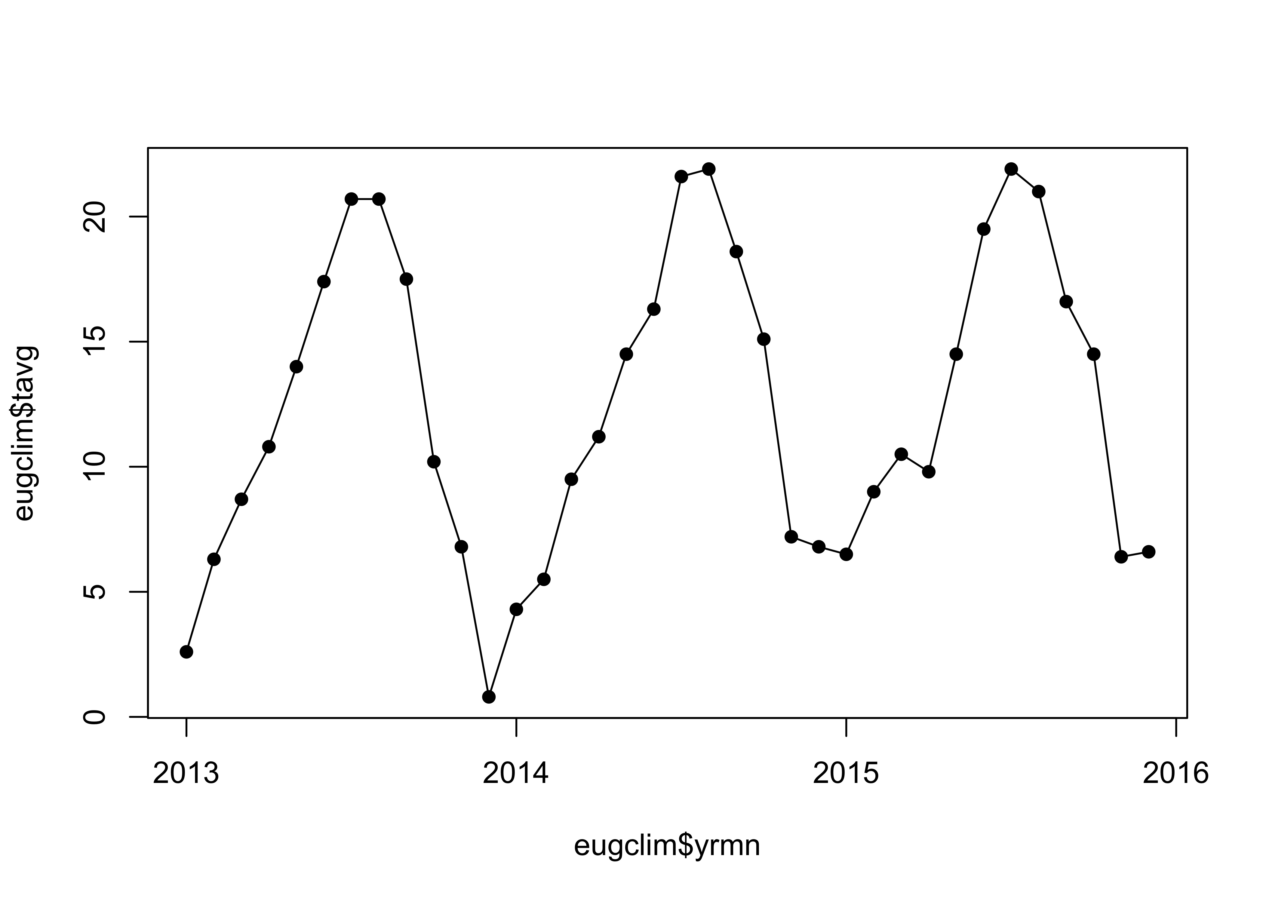

[Back to top]

3 A data-wrangling example

An alternative way in which that Eugene climate data could have been laid out is one in which there are blocks of data, one per year, with months in columns, and individual variables in rows:

# alternative layout
csv_file <- "/Users/bartlein/Documents/geog495/data/csv/EugeneClim-short-alt-tvars.csv"
eugclim_alt <- read_csv(csv_file)

## Parsed with column specification:
## cols(
##   year = col_double(),
##   param = col_character(),
##   `1` = col_double(),
##   `2` = col_double(),
##   `3` = col_double(),
##   `4` = col_double(),
##   `5` = col_double(),
##   `6` = col_double(),
##   `7` = col_double(),
##   `8` = col_double(),
##   `9` = col_double(),
##   `10` = col_double(),
##   `11` = col_double(),
##   `12` = col_double()
## )

eugclim_alt

## # A tibble: 15 x 14
##     year param   `1`   `2`   `3`   `4`   `5`   `6`   `7`   `8`   `9`  `10`  `11`  `12`
##    <dbl> <chr> <dbl> <dbl> <dbl> <dbl> <dbl> <dbl> <dbl> <dbl> <dbl> <dbl> <dbl> <dbl>
##  1  2013 tmax    5.7  10.2  14.5  17    21.1  25    30.6  28.6  23.1  16.5  11.1   4.9
##  2  2013 tmin   -0.4   2.3   3     4.6   6.9   9.8  10.8  12.7  11.9   3.9   2.6  -3.2
##  3  2013 tavg    2.6   6.3   8.7  10.8  14    17.4  20.7  20.7  17.5  10.2   6.8   0.8
##  4  2013 emxt   13.3  13.9  22.2  25.6  30    35.6  35.6  35    32.2  25.6  17.8  13.3
##  5  2013 emnt   -6.7  -2.8  -2.2  -0.5   1.1   4.4   6.1   7.8   5    -2.1  -7.1 -23.2
##  6  2014 tmax    7.8   9.1  14.9  17.4  21.7  23.8  30.9  31    27.2  21.2  11.3  10  
##  7  2014 tmin    0.8   1.9   4.1   5     7.3   8.8  12.3  12.8  10.1   9     3.2   3.6
##  8  2014 tavg    4.3   5.5   9.5  11.2  14.5  16.3  21.6  21.9  18.6  15.1   7.2   6.8
##  9  2014 emxt   13.3  17.2  23.3  27.8  31.1  29.4  36.1  38.3  36.7  30    19.4  16.7
## 10  2014 emnt   -4.3  -6.6  -2.1   1.1   1.7   3.9   8.3   7.2   6.1   4.4  -6.6  -7.1
## 11  2015 tmax   10.4  13.8  17    16.6  21.2  28.7  31.2  29.9  25    21.4  11.3   9.5
## 12  2015 tmin    2.6   4.2   4     3     7.9  10.4  12.6  12.2   8.1   7.6   1.4   3.7
## 13  2015 tavg    6.5   9    10.5   9.8  14.5  19.5  21.9  21    16.6  14.5   6.4   6.6
## 14  2015 emxt   20    18.3  22.2  25    29.4  36.7  40.6  37.8  33.9  28.9  18.3  16.7
## 15  2015 emnt   -6    -3.2  -3.2   0.6   2.2   5     8.3   7.2   3.3   0.6  -8.2  -4.3

This layout is obviously not “tidy”, but is not atypical of the way many data sets are provided. With considerable cutting and pasting in Excel (including transposing data using Paste > Special) these data could be rearranged, but such editing is prone to mistakes, masks what has actually been done to the data, and is not easy to repeat.

3.1 Reshaping by gathering

The data can be reshaped into the appropriate form using the gather() function in the tidyr package. To illustrate this, first make another data set that includes just the average temperature data (tavg) from the “untidy” version of the data:

# get just the tavg data
eugclim_alt_tavg <- eugclim_alt[eugclim_alt$param == "tavg", ]
eugclim_alt_tavg

## # A tibble: 3 x 14
##    year param   `1`   `2`   `3`   `4`   `5`   `6`   `7`   `8`   `9`  `10`  `11`  `12`
##   <dbl> <chr> <dbl> <dbl> <dbl> <dbl> <dbl> <dbl> <dbl> <dbl> <dbl> <dbl> <dbl> <dbl>
## 1  2013 tavg    2.6   6.3   8.7  10.8  14    17.4  20.7  20.7  17.5  10.2   6.8   0.8
## 2  2014 tavg    4.3   5.5   9.5  11.2  14.5  16.3  21.6  21.9  18.6  15.1   7.2   6.8
## 3  2015 tavg    6.5   9    10.5   9.8  14.5  19.5  21.9  21    16.6  14.5   6.4   6.6

Then reshape the data using gather():

# reshape by gathering
eugclim_alt_tavg2 <- gather(eugclim_alt_tavg, `1`:`12`, key="month", value="cases")
eugclim_alt_tavg2

## # A tibble: 36 x 4
##     year param month cases
##    <dbl> <chr> <chr> <dbl>
##  1  2013 tavg  1       2.6
##  2  2014 tavg  1       4.3
##  3  2015 tavg  1       6.5
##  4  2013 tavg  2       6.3
##  5  2014 tavg  2       5.5
##  6  2015 tavg  2       9  
##  7  2013 tavg  3       8.7
##  8  2014 tavg  3       9.5
##  9  2015 tavg  3      10.5
## 10  2013 tavg  4      10.8
## # … with 26 more rows

The arguments of the gather() function include 1) the table to be reshaped (eugclim_alt_tavg), 2) the columns to be gathered together (here specified as `1`:`12` and note the use of the backtick (`) to indicate the columnn names, which in this example are character (chr) variables), 3) the “key” column that individual columns will be stacked up into, and 4) the values that will be stacked.

The observations are not quite in the right time-series order, but they can be sorted using the arrange() function from the dplyr package:

# rearrange (sort)
eugclim_alt_tavg3 <- arrange(eugclim_alt_tavg2, year)
eugclim_alt_tavg3

## # A tibble: 36 x 4
##     year param month cases
##    <dbl> <chr> <chr> <dbl>
##  1  2013 tavg  1       2.6
##  2  2013 tavg  2       6.3
##  3  2013 tavg  3       8.7
##  4  2013 tavg  4      10.8
##  5  2013 tavg  5      14  
##  6  2013 tavg  6      17.4
##  7  2013 tavg  7      20.7
##  8  2013 tavg  8      20.7
##  9  2013 tavg  9      17.5
## 10  2013 tavg  10     10.2
## # … with 26 more rows

Add a decimal year (yrmn) variable to the new data set, and plot.

# add decimal year value
eugclim_alt_tavg3$yrmn <- eugclim_alt_tavg3$year + (as.integer(eugclim_alt_tavg3$month)-1)/12
plot(eugclim_alt_tavg3$cases ~ eugclim_alt_tavg3$yrmn, type="o", pch=16, col="blue", xaxp=c(2013, 2016, 3))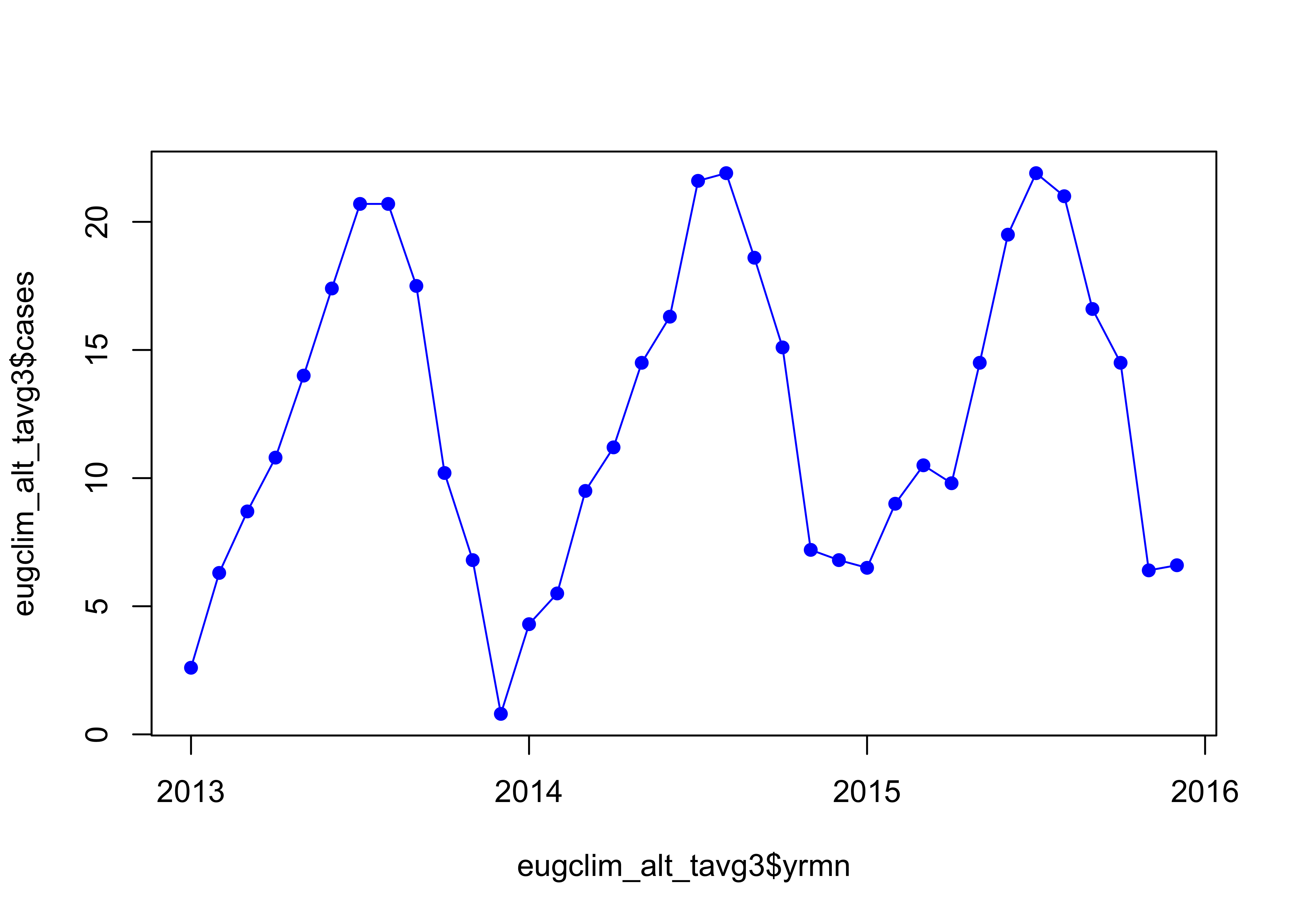

Looks right.

3.2 Reshape the whole data set

The whole alternative-layout data set can be reshaped by first gathering the data

# alternative layout -- gather, then spread
eugclim_alt2 <- gather(eugclim_alt, `1`:`12`, key="month", value="cases")
eugclim_alt2

## # A tibble: 180 x 4
##     year param month cases
##    <dbl> <chr> <chr> <dbl>
##  1  2013 tmax  1       5.7
##  2  2013 tmin  1      -0.4
##  3  2013 tavg  1       2.6
##  4  2013 emxt  1      13.3
##  5  2013 emnt  1      -6.7
##  6  2014 tmax  1       7.8
##  7  2014 tmin  1       0.8
##  8  2014 tavg  1       4.3
##  9  2014 emxt  1      13.3
## 10  2014 emnt  1      -4.3
## # … with 170 more rows

The month values, which are now characters (which just happen to be numerals here), can be recoded to integers as follows:

# convert integer to month
eugclim_alt2$month <- as.integer(eugclim_alt2$month)

Then the “tall” stack of data is spread into rectangular data set using the values in the param column:

# spread
eugclim_alt3 <- spread(eugclim_alt2, key="param", value=cases)
eugclim_alt3

## # A tibble: 36 x 7
##     year month  emnt  emxt  tavg  tmax  tmin
##    <dbl> <int> <dbl> <dbl> <dbl> <dbl> <dbl>
##  1  2013     1  -6.7  13.3   2.6   5.7  -0.4
##  2  2013     2  -2.8  13.9   6.3  10.2   2.3
##  3  2013     3  -2.2  22.2   8.7  14.5   3  
##  4  2013     4  -0.5  25.6  10.8  17     4.6
##  5  2013     5   1.1  30    14    21.1   6.9
##  6  2013     6   4.4  35.6  17.4  25     9.8
##  7  2013     7   6.1  35.6  20.7  30.6  10.8
##  8  2013     8   7.8  35    20.7  28.6  12.7
##  9  2013     9   5    32.2  17.5  23.1  11.9
## 10  2013    10  -2.1  25.6  10.2  16.5   3.9
## # … with 26 more rows

Plot the reshaped data:

# plot the reshapted data
eugclim_alt3$yrmn <- eugclim_alt3$year + (as.integer(eugclim_alt3$month)-1)/12
plot(eugclim_alt3$tavg ~ eugclim_alt3$yrmn, type="o", pch=16, col="red", xaxp=c(2013, 2016, 3))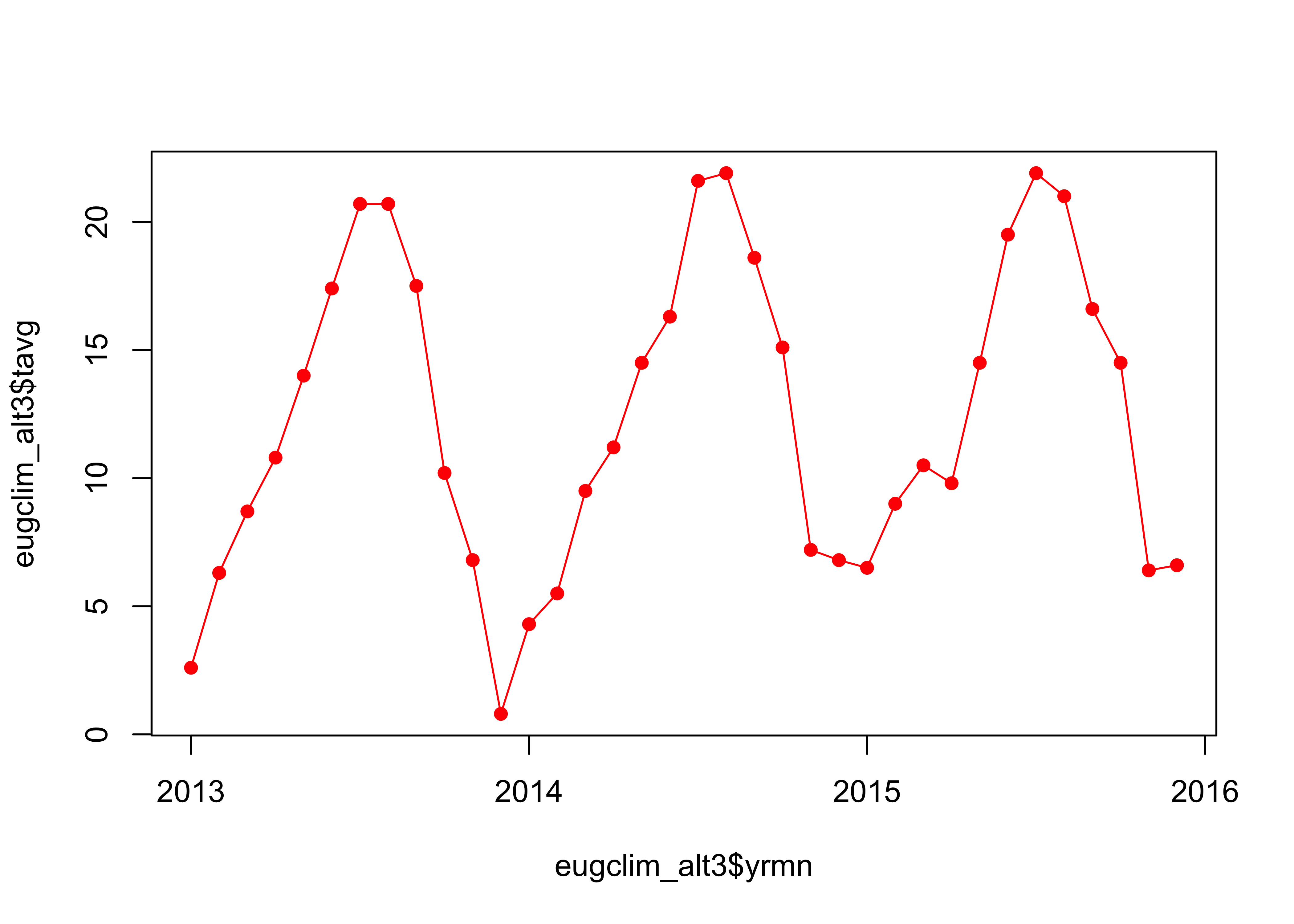

[Back to top]

4 Other data-wrangling tasks

There are a number of other operations on a data table using the dplyr package (as well as base R) that can produce useful results.

4.1 Summarization

Summarize the whole data set. In this example, summarize_all() generates a long-term mean of the data.

# summarize
eugclim_ltm <- summarize_all(eugclim, "mean")
eugclim_ltm

## # A tibble: 1 x 18
##    year   mon  yrmn  tmax  tmin  tavg  emxt   emnt  htdd  cldd  prcp  emxp  dp01  dp05  dp10  snow  emsd
##   <dbl> <dbl> <dbl> <dbl> <dbl> <dbl> <dbl>  <dbl> <dbl> <dbl> <dbl> <dbl> <dbl> <dbl> <dbl> <dbl> <dbl>
## 1  2014   6.5 2014.  18.6  6.15  12.4  26.3 -0.331  201.  20.9  66.9  17.3  11.1  1.64 0.417    NA    NA
## # … with 1 more variable: awnd <dbl>

Filter out just the January values, and get a long-term mean of those:

# filter
eugclim_jan <- filter(eugclim, mon==1)
eugclim_jan

## # A tibble: 3 x 18
##    year   mon  yrmn  tmax  tmin  tavg  emxt  emnt  htdd  cldd  prcp  emxp  dp01  dp05  dp10  snow  emsd
##   <dbl> <dbl> <dbl> <dbl> <dbl> <dbl> <dbl> <dbl> <dbl> <dbl> <dbl> <dbl> <dbl> <dbl> <dbl> <dbl> <dbl>
## 1  2013     1  2013   5.7  -0.4   2.6  13.3  -6.7  487.     0  34.5   6.4    11     0     0    NA    NA
## 2  2014     1  2014   7.8   0.8   4.3  13.3  -4.3  436.     0  65.4  17.5    11     2     0    NA     0
## 3  2015     1  2015  10.4   2.6   6.5  20    -6    368.     0  60.7  33.8    10     2     1    NA     0
## # … with 1 more variable: awnd <dbl>

eugclim_jan_ltm <- summarize_all(eugclim_jan, "mean")
eugclim_jan_ltm

## # A tibble: 1 x 18
##    year   mon  yrmn  tmax  tmin  tavg  emxt  emnt  htdd  cldd  prcp  emxp  dp01  dp05  dp10  snow  emsd
##   <dbl> <dbl> <dbl> <dbl> <dbl> <dbl> <dbl> <dbl> <dbl> <dbl> <dbl> <dbl> <dbl> <dbl> <dbl> <dbl> <dbl>
## 1  2014     1  2014  7.97     1  4.47  15.5 -5.67  430.     0  53.5  19.2  10.7  1.33 0.333    NA    NA
## # … with 1 more variable: awnd <dbl>

Summarize the data by groups, in this case by months. First rearrange the data, and then summarize:

# summarize by groups -- define groups
eugclim_group <- group_by(eugclim, mon)
eugclim_group

## # A tibble: 36 x 18
## # Groups:   mon [12]
##     year   mon  yrmn  tmax  tmin  tavg  emxt  emnt  htdd  cldd  prcp  emxp  dp01  dp05  dp10  snow  emsd
##    <dbl> <dbl> <dbl> <dbl> <dbl> <dbl> <dbl> <dbl> <dbl> <dbl> <dbl> <dbl> <dbl> <dbl> <dbl> <dbl> <dbl>
##  1  2013     1 2013    5.7  -0.4   2.6  13.3  -6.7 487.    0    34.5   6.4    11     0     0    NA    NA
##  2  2013     2 2013.  10.2   2.3   6.3  13.9  -2.8 338.    0    41    11.2    14     0     0    NA    NA
##  3  2013     3 2013.  14.5   3     8.7  22.2  -2.2 298.    0    54.2  12.7    12     1     0    NA    NA
##  4  2013     4 2013.  17     4.6  10.8  25.6  -0.5 226.    0    36.8  11.9    10     0     0    NA     0
##  5  2013     5 2013.  21.1   6.9  14    30     1.1 137.    2.5  51.7  13      13     1     0    NA     0
##  6  2013     6 2013.  25     9.8  17.4  35.6   4.4  54    25.3  28.1  18.3     7     1     0     0     0
##  7  2013     7 2014.  30.6  10.8  20.7  35.6   6.1   4.5  77.7   0     0       0     0     0     0     0
##  8  2013     8 2014.  28.6  12.7  20.7  35     7.8   7.1  79.2   6.4   3.8     4     0     0     0     0
##  9  2013     9 2014.  23.1  11.9  17.5  32.2   5    57    33.1 180.   48.3    15     6     1    NA     0
## 10  2013    10 2014.  16.5   3.9  10.2  25.6  -2.1 252.    0    14.8   8.4     6     0     0    NA     0
## # … with 26 more rows, and 1 more variable: awnd <dbl>

Note that grouped data set looks almost exactly like the ungrouped one, except when listed, it includes the mention of the grouping variable (i.e., Groups: mon [12]).

# summarize groups
eugclim_summary <- summarize_all(eugclim_group, list(mean = mean))
eugclim_summary

## # A tibble: 12 x 18
##      mon year_mean yrmn_mean tmax_mean tmin_mean tavg_mean emxt_mean emnt_mean htdd_mean cldd_mean
##    <dbl>     <dbl>     <dbl>     <dbl>     <dbl>     <dbl>     <dbl>     <dbl>     <dbl>     <dbl>
##  1     1      2014     2014       7.97      1         4.47      15.5    -5.67     430.        0   
##  2     2      2014     2014.     11.0       2.8       6.93      16.5    -4.2      320.        0   
##  3     3      2014     2014.     15.5       3.7       9.57      22.6    -2.5      271.        0   
##  4     4      2014     2014.     17         4.2      10.6       26.1     0.4      232.        0   
##  5     5      2014     2014.     21.3       7.37     14.3       30.2     1.67     125.        2.03
##  6     6      2014     2014.     25.8       9.67     17.7       33.9     4.43      47.3      29.4 
##  7     7      2014     2014.     30.9      11.9      21.4       37.4     7.57       3.73     98.7 
##  8     8      2014     2015.     29.8      12.6      21.2       37.0     7.4        3.13     91.8 
##  9     9      2014     2015.     25.1      10.0      17.6       34.3     4.8       49.2      26.5 
## 10    10      2014     2015.     19.7       6.83     13.3       28.2     0.967    159.        2.03
## 11    11      2014     2015.     11.2       2.4       6.8       18.5    -7.3      346.        0   
## 12    12      2014     2015.      8.13      1.37      4.73      15.6   -11.5      421         0   
## # … with 8 more variables: prcp_mean <dbl>, emxp_mean <dbl>, dp01_mean <dbl>, dp05_mean <dbl>,
## #   dp10_mean <dbl>, snow_mean <dbl>, emsd_mean <dbl>, awnd_mean <dbl>

Calculate annual averages of each variable, using the aggregate() function from the stats package.

# aggregate
eugclim_ann <- aggregate(eugclim, by=list(eugclim$year), FUN="mean")
eugclim_ann

##   Group.1 year mon     yrmn     tmax     tmin     tavg     emxt       emnt     htdd     cldd     prcp
## 1    2013 2013 6.5 2013.458 17.35833 5.408333 11.37500 25.00833 -1.6833333 229.0083 18.15000 44.93333
## 2    2014 2014 6.5 2014.458 18.85833 6.575000 12.70833 26.60833  0.5000000 190.2500 20.95000 87.46667
## 3    2015 2015 6.5 2015.458 19.66667 6.475000 13.06667 27.31667  0.1916667 182.5500 23.53333 68.32500
##       emxp     dp01      dp05       dp10 snow     emsd     awnd
## 1 13.36667  9.50000 0.9166667 0.08333333   NA       NA 2.525000
## 2 21.49167 13.25000 2.2500000 0.58333333   NA 14.83333 3.033333
## 3 17.18333 10.41667 1.7500000 0.58333333   NA  0.00000 2.958333

4.2 The pipe operator

Operations on a data table that require multiple steps can be streamlined both in appearance in the code and in the operations themselves using the “Pipe” operator (%>%) from the magrittr package. The operator “pipes”, or moves forward, the output from one function to another.

Here’s a simple example, combining the grouping and summarization steps for calculating means by month.

# the pipe
eugclim_summary <- eugclim %>% group_by(mon) %>% summarize_all(funs("mean"))
eugclim_summary

## # A tibble: 12 x 18
##      mon  year  yrmn  tmax  tmin  tavg  emxt    emnt   htdd  cldd   prcp  emxp  dp01  dp05  dp10  snow
##    <dbl> <dbl> <dbl> <dbl> <dbl> <dbl> <dbl>   <dbl>  <dbl> <dbl>  <dbl> <dbl> <dbl> <dbl> <dbl> <dbl>
##  1     1  2014 2014   7.97  1     4.47  15.5  -5.67  430.    0     53.5  19.2  10.7  1.33  0.333    NA
##  2     2  2014 2014. 11.0   2.8   6.93  16.5  -4.2   320.    0    116.   22.9  15.7  3.33  1        NA
##  3     3  2014 2014. 15.5   3.7   9.57  22.6  -2.5   271.    0    100.   21.4  14.3  3     0.667    NA
##  4     4  2014 2014. 17     4.2  10.6   26.1   0.4   232.    0     45.3  10.4  12.3  0     0        NA
##  5     5  2014 2014. 21.3   7.37 14.3   30.2   1.67  125.    2.03  39.2  10.7  12.3  0.333 0        NA
##  6     6  2014 2014. 25.8   9.67 17.7   33.9   4.43   47.3  29.4   22.2  13.5   6    0.667 0         0
##  7     7  2014 2014. 30.9  11.9  21.4   37.4   7.57    3.73 98.7    3.6   2.03  2.33 0     0         0
##  8     8  2014 2015. 29.8  12.6  21.2   37.0   7.4     3.13 91.8    5.73  3.63  3.33 0     0         0
##  9     9  2014 2015. 25.1  10.0  17.6   34.3   4.8    49.2  26.5   77.0  26.2  10    2.33  0.333    NA
## 10    10  2014 2015. 19.7   6.83 13.3   28.2   0.967 159.    2.03  65.5  22.7  11.7  1     0.667    NA
## 11    11  2014 2015. 11.2   2.4   6.8   18.5  -7.3   346.    0     86.5  22.8  15    1.67  0.333    NA
## 12    12  2014 2015.  8.13  1.37  4.73  15.6 -11.5   421     0    188.   32.7  19    6     1.67     NA
## # … with 2 more variables: emsd <dbl>, awnd <dbl>

What happens here is that the data table eugclim, is passed forward into the group_by() function, and the output from that is passed into the summarize_all() function. There is, of course, a tradeoff between the explicitness of doing one thing at a time, and the efficiency of a single line of code that performs multiple operations.

4.3 Calculating anomalies

A common task in analyzing climate data is to convert the “absolute” values (i.e. the observations) into “anomalies” or deviations from some long-term mean (and note that “absolute values” here should not be confused with those unsigned values of a variable produced by the absolute-value operator abs(), e.g. |x|).

# anomalies
eugclim$tavg_anm <- eugclim$tavg - eugclim_summary$tavg
eugclim$tavg_anm

##  [1] -1.86666667 -0.63333333 -0.86666667  0.20000000 -0.33333333 -0.33333333 -0.70000000 -0.50000000
##  [9] -0.06666667 -3.06666667  0.00000000 -3.93333333 -0.16666667 -1.43333333 -0.06666667  0.60000000
## [17]  0.16666667 -1.43333333  0.20000000  0.70000000  1.03333333  1.83333333  0.40000000  2.06666667
## [25]  2.03333333  2.06666667  0.93333333 -0.80000000  0.16666667  1.76666667  0.50000000 -0.20000000
## [33] -0.96666667  1.23333333 -0.40000000  1.86666667

Plot the anomalies.

# plot anomalies
plot(eugclim$tavg_anm ~ eugclim$yrmn, type="o", pch=16, col="green", xaxp=c(2013, 2016, 3))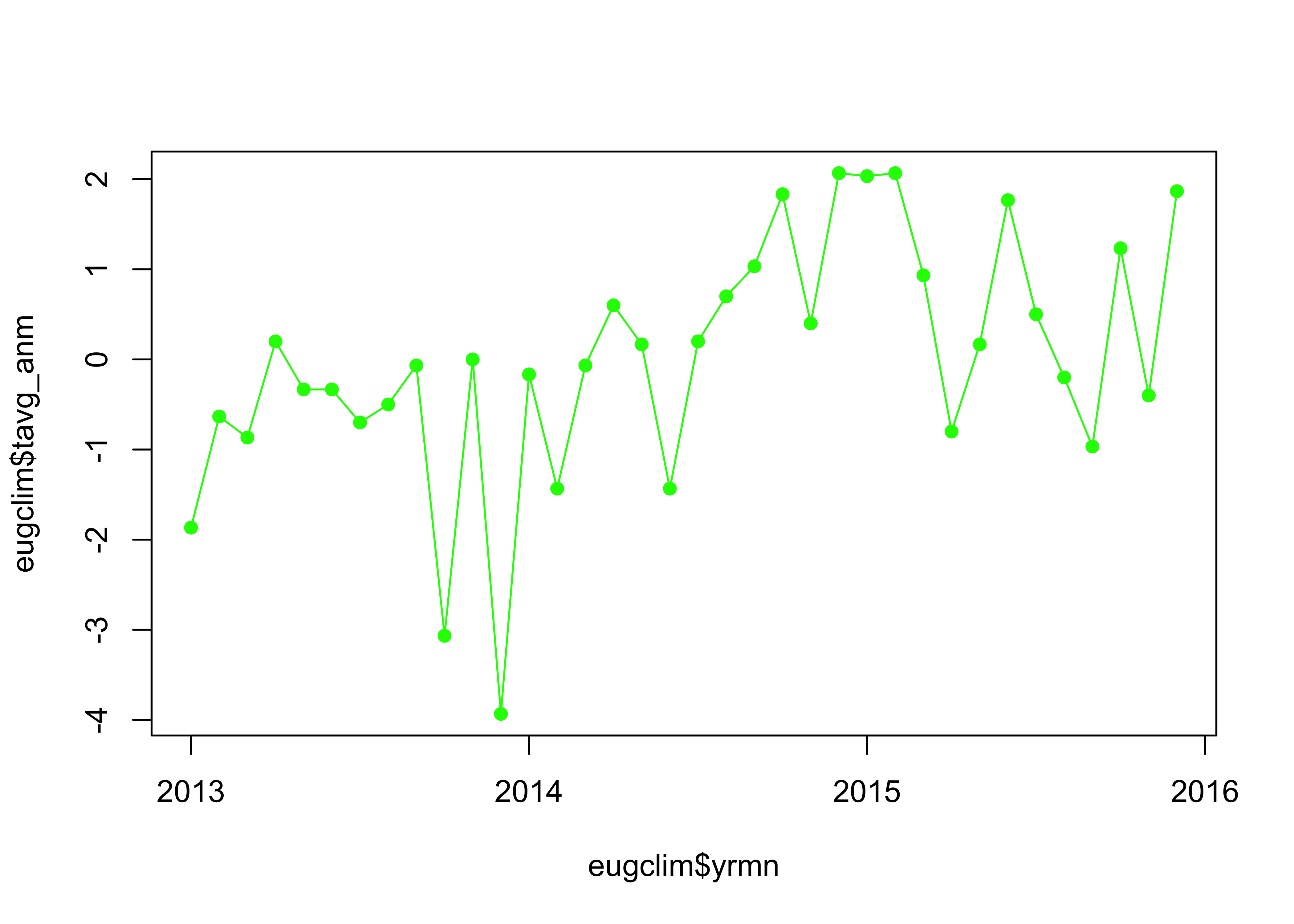

[Back to top]

5 Matrix algebra

Matrix algebra provides an elegant way of representing both the data the kind of operations on tables or arrays that frequently come up in data analysis, and when implemented numerically, matrix algebra also provides efficient an means of carrying those operations out. The following is a brief introduction to matrix algebra as implmented in R.

A short dicussion of matrices in general, special matrices, and matrix operations can be found here: matrix.pdf

5.1 Some basic matrix definitions in R

Create the 3 row by 2 column matrix A. Note the use of the concatenation (c()) function to collect the individual matrix elements (the a_ij’s) together, and the default fill order (byrow = FALSE), which implies filling the matrix by rows:

# create a matrix
# default fill method: byrow = FALSE
A <- matrix(c(6, 9, 12, 13, 21, 5), nrow=3, ncol=2)
A

##      [,1] [,2]
## [1,]    6   13
## [2,]    9   21
## [3,]   12    5

class(A)

## [1] "matrix"

The class() function indicates that A is indeed a matrix (as opposed to a data frame).

Create another matrix, B, with the same elements, only filled by row this time:

# same elements, but byrow = TRUE
B <-  matrix(c(6, 9, 12, 13, 21, 5), nrow=3, ncol=2, byrow=TRUE)
B

##      [,1] [,2]
## [1,]    6    9
## [2,]   12   13
## [3,]   21    5

Individual matrix elements can be reference using the “square-bracket selection” rules.

# referencing matrix elements
A[1,2] # row 1, col 2

## [1] 13

A[2,1] # row 2, col 1

## [1] 9

A[2, ] # all elements in row 2

## [1]  9 21

A[, 2] # all elements in column 2 ] 

## [1] 13 21  5

For comparison, create a vector c:

# create a vector
c <- c(1,2,3,4,5,6,7,8,9)
c

## [1] 1 2 3 4 5 6 7 8 9

class(c)

## [1] "numeric"

At this point, c is just a list of numbers. The as.matrix() function creates a 9 row by 1 column vector, which can be verified by the dim() function:

c <- as.matrix(c)
class(c)

## [1] "matrix"

dim(c)

## [1] 9 1

The vector c has 9 rows and 1 column.

A vector can be reshaped into a matrix:

# reshape the vector into a 3x3 matrix
C <- matrix(c, nrow=3, ncol=3)
C

##      [,1] [,2] [,3]
## [1,]    1    4    7
## [2,]    2    5    8
## [3,]    3    6    9

A vector can also be created from a single row or column of a matrix:

# create a vector from a column or row of a matrix
a1 <- as.matrix(A[, 1]) # vector from column 1
a1

##      [,1]
## [1,]    6
## [2,]    9
## [3,]   12

dim(a1)

## [1] 3 1

a1 is a 3 row by 1 column column vector.

5.2 Matrix operations

Transposition (t()) flips the rows and columns of a matrix:

# transposition
A

##      [,1] [,2]
## [1,]    6   13
## [2,]    9   21
## [3,]   12    5

t(A)

##      [,1] [,2] [,3]
## [1,]    6    9   12
## [2,]   13   21    5

A second example, the transpose of C

C

##      [,1] [,2] [,3]
## [1,]    1    4    7
## [2,]    2    5    8
## [3,]    3    6    9

t(C)

##      [,1] [,2] [,3]
## [1,]    1    2    3
## [2,]    4    5    6
## [3,]    7    8    9

Vectors and also be transposed, which simply turns a column vector, e.g. a1 into a row vector

a1t <- t(a1)
a1t

##      [,1] [,2] [,3]
## [1,]    6    9   12

dim(a1t)

## [1] 1 3

5.3 Matrix algebra

Matrix algebra is basically analogous to scalar algebra (with the exception of division), and obeys most of the same rules that scalar algebra does.

Add two matrices, A and B:

# addition
F <- A + B
F

##      [,1] [,2]
## [1,]   12   22
## [2,]   21   34
## [3,]   33   10

Note that the individual elements of A and B are simply added together to produce the corresponding elements of F (i.e. f_ij = a_ij + b_ij).

In order to be added together, the matrices have to be of the same shape (i.e. have the same number of rows and colums). The shape of a matrix can be verified using the dim() function:

dim(C)

## [1] 3 3

dim(A)

## [1] 3 2

Here, A and C are not the same shape, and the following code, if executed, would product an error message:

# A and C not same shape
G <- A + C

Scalar multiplication involves muliplying each element of a matrix by a scalar value:

# scalar multiplication
H <- 0.5*A
H

##      [,1] [,2]
## [1,]  3.0  6.5
## [2,]  4.5 10.5
## [3,]  6.0  2.5

Here, h_ij = 0.5 · a_ij. Element-by-element multiplication is also possible for identically shaped matrices, e.g., p_ij = a_ij · b_ij:

# element-by-element multipliction
P <- A*B
P

##      [,1] [,2]
## [1,]   36  117
## [2,]  108  273
## [3,]  252   25

5.3.1 Matrix multiplication

Matrix multiplication (see matrix.pdf) results in a a set of sums and crossproducts, as opposed to element-by-element products. Matrix multiplication is symbolized by the %*% operator:

# matrix multiplication
Q <- C %*% A
Q

##      [,1] [,2]
## [1,]  126  132
## [2,]  153  171
## [3,]  180  210

dim(C); dim(A)

## [1] 3 3

## [1] 3 2

Note that the matrices have to be conformable, as they are here (the number of columns of the first matrix must equal the number of rows of the second, and the product matrix Q here has the number of rows of the first matrix and the number of columns of the second).

The matrices A and B are not conformable for multiplication; although they have the same shape, they are not square, and the following code would produce an error:

T <- A %*% B # not conformable

dim(A); dim(B)

## [1] 3 2

## [1] 3 2

5.4 Special matrices

There are a number of special matrices that come up in data analysis. Here D is a diagonal matrix, with non-zero values along the principal diagonal, and zeros elsewhere:

# diagonal matrix
D <- diag(c(6,2,1,3), nrow=4, ncol=4)
D

##      [,1] [,2] [,3] [,4]
## [1,]    6    0    0    0
## [2,]    0    2    0    0
## [3,]    0    0    1    0
## [4,]    0    0    0    3

A special form of a diagonal matrix is the identity matrix I, which has ones along the principal diagonal, and zeros elsewhere:

# identity matrix
I <- diag(1, nrow=4, ncol=4)
I

##      [,1] [,2] [,3] [,4]
## [1,]    1    0    0    0
## [2,]    0    1    0    0
## [3,]    0    0    1    0
## [4,]    0    0    0    1

A special scalar that appears often in practice is the norm (or Euclidean norm) of a vector, which is simply the square root of the sum of squares of the elements of the vector:

# Euclidean norm of a vector
anorm <- sqrt(t(a1) %*% a1)
anorm

##          [,1]
## [1,] 16.15549

It can be verified that sqrt(sum(a1^2)) = 16.1554944.

5.4.1 Inverse matrices

The matrix algebra equivalent of division is the multiplication of one matrix by the inverse of another. To illustrate this, and the topic of the eigenstructure of a matrix discussed below, we can look at a realistic matrix, the correlation matrix of the temperature variables in the Oregon climate-station data set.

Here’s the correlation matrix, R:

# a realistic matrix, orstationc temperature-variable correlation matrix
R <- cor(cbind(orstationc$tjan, orstationc$tjul, orstationc$tann))
R

##            [,1]       [,2]      [,3]
## [1,]  1.0000000 -0.3639314 0.7253877
## [2,] -0.3639314  1.0000000 0.3641966
## [3,]  0.7253877  0.3641966 1.0000000

The inverse of the correlation matrix R, written as R^-1 is obtained using the solve() function:

# matrix inversion
Rinv <- solve(R)
Rinv

##           [,1]      [,2]      [,3]
## [1,]  52.76560  38.21117 -52.19190
## [2,]  38.21117  28.82424 -38.21560
## [3,] -52.19190 -38.21560  52.77735

As in scalar division, where a · (1/a) = 1.0, postmuliplying a matrix by its inverse yields the Identity matrix, I:

# check inverse
D <- R %*% Rinv
D

##              [,1]         [,2]          [,3]
## [1,] 1.000000e+00 3.552714e-15  0.000000e+00
## [2,] 3.552714e-15 1.000000e+00 -7.105427e-15
## [3,] 7.105427e-15 7.105427e-15  1.000000e+00

After rounding using the zapsmall() function D indeed equals I:

zapsmall(D)

##      [,1] [,2] [,3]
## [1,]    1    0    0
## [2,]    0    1    0
## [3,]    0    0    1

5.4.2 Eigenvectors and eigenvalues

An important concept that comes up in multivariate analysis is the decomposition of a matrix like the correlation matrix R (see matrix.pdf), into another square matrix, E, and a diagonal matrix, V, that each have some desireable properties, and which make the following statement true: RE = EV, where V is a diagonal matrix with the elements v_i along the diagonal. The matrix E contains the eigenvectors of R, while the v_i’s are the eigenvalues of R.

# eigenvectors
E <- eigen(R)
E

## eigen() decomposition
## $values
## [1] 1.725387748 1.267093364 0.007518887
## 
## $vectors
##            [,1]       [,2]       [,3]
## [1,] 0.70702003 -0.3258720 -0.6276385
## [2,] 0.00034552  0.8876651 -0.4604894
## [3,] 0.70719344  0.3253584  0.6277096

[Back to top]

6 Readings

• Data wrangling is nicely covered in the “preprint” version of the R for Data Science book by Wickham and Grolemund (2017), available at http://r4ds.had.co.nz or through the Bookdown web site at https://bookdown.org

• Irizarry (Intro to Data Science): Ch. 3, 4, 20, 21

The routines used in data wrangling are covered in the following cheatsheets from the RStudio web site:

• Data Import with readr, tibble, and tidyr
• Data Transformation with dplyr
• Data Wrangling with dplyr and tidyr, a previous version of the above.

Matrix algebra is concisely reviewed in:

Rencher, A., 2002, Matrix Algebra, Ch. 2 in Methods of Multivariate Analysis, Wiley. The chapter (and book) is available online through http://library.uoregon.edu.