1 Introduction

This script (binboot-curve.R) fits step-like composite curves, with bootstrapping by site confidence intervals, via binning. As is the case with other analysis scripts, the script has two parts, a set-up portion that changes from analysis to analysis, and a computation part that does not change. This version reads “presampled” data.

2 Set up

The variables queryname, basename and binname are used to compose the path and filenames for the presampled data.

# age-bin averages of influx data
# bootstrap-by-site confidence intervals

# names
queryname <- "v3i" # 
basename <- "nt2kb" 

# paths for input and output .csv files -- modify as appropriate
datapath <- "/Projects/GPWG/GPWGv3/GCDv3Data/v3i/"
sitelistpath <- "/Projects/GPWG/GPWGv3/GCDv3Data/v3i/v3i_sitelists/"
sitelist <- "v3i_nsa_globe"
outpath <- "/Projects/GPWG/GPWGv3/GCDv3Data/v3i/v3i_curves/"

# prebinning bin width
pbw <- 10

pbw_char <- as.character(pbw)
if (pbw < 10) pbw_char <- paste("0", pbw_char, sep="")

Set the number of bootstrap samples or replications:

# number of bootstrap samples/replications
nreps <- 200

Specifiy the age-bin centers, and spacing. This version uses 20-year wide bins, with the first bin centered at -60 yr BP, or 2010 CE, and the last at 1950 yr BP, or 1 CE.

# age bin centers
abw <- 20 
abinbeg <- -60 
abinend <- 1950

Set array sizes for saving bootstrap results.

# array sizes
maxrecs <- 2000
maxreps <- 1000

# plotting set up
xmin <- 0; xmax <- 2020; ymin1 <- -1.0; ymax1 <- 1.0; ymin2 <- -0.5; ymax2 <- 1.0
xlim=c(xmin,xmax); ylim1=c(ymin1,ymax1); ylim2 <- c(ymin2,ymax2)
xlab="Year CE"; xminortick <- 50
ylab="Normalized Anomalies of Transformed Influx"

# plot output 
plotout <- "screen" # "pdf" # "png" #

3 Calculation preliminaries

3.1 Initial steps

Set various output paths and filenames.

# no changes below here

# prebinning file name
binname <- paste("bw", pbw_char, sep="")

# presampled/binned files
csvpath <- "/Projects/GPWG/GPWGv3/GCDv3Data/v3i/v3i_presamp_csv/"
csvname <- paste("_presamp_influx_",basename,"_",binname,".csv", sep="")

# site list file
sitelistfile <- paste(sitelistpath, sitelist, ".csv", sep="")
sitelistfile

## [1] "/Projects/GPWG/GPWGv3/GCDv3Data/v3i/v3i_sitelists/v3i_nsa_globe.csv"

# curve (output) path and file
curvecsvpath <- paste(datapath,queryname,"_curves/",sep="")

# if output folder does not exist, create it
dir.create(file.path(datapath, paste(queryname,"_curves/",sep="")), showWarnings=FALSE)
curvename <- paste(sitelist,"_binboot_",basename,"_",binname,"_abw",as.character(abw),"_",
  as.character(nreps), sep="")
curvefile <- paste(curvename, ".csv", sep="")
print(curvecsvpath)

## [1] "/Projects/GPWG/GPWGv3/GCDv3Data/v3i/v3i_curves/"

print(curvename)

## [1] "v3i_nsa_globe_binboot_nt2kb_bw10_abw20_200"

print(curvefile)

## [1] "v3i_nsa_globe_binboot_nt2kb_bw10_abw20_200.csv"

Code block to implement writing .pdf to file:

# .pdf plot of bootstrap iterations
if (plotout == "pdf") {
pdffile <- paste(curvename, ".pdf", sep="")
print(pdffile)
}
# .png plot of bootstrap iterations
if (plotout == "png") {
  pngfile <- paste(curvename, ".png", sep="")
  print(pngfile)
}

Read the list of sites to be processed. Note that this is the site list may contain sites that after transforming and presampling may have no useful data. Those sites are ignored when the data are read in.

# read the list of sites
sites <- read.csv(sitelistfile)
head(sites)

##   Site_ID     Lat       Lon Elev depo_context         Site_Name
## 1       1 44.6628 -110.6161 2530         LASE            Cygnet
## 2       2 44.9183 -110.3467 1884         LASE Slough Creek Pond
## 3       3 45.7044 -114.9867 2250         LASE        Burnt Knob
## 4       4 45.8919 -114.2619 2300         LASE             Baker
## 5       5 46.3206 -114.6503 1770         LASE            Hoodoo
## 6       6 45.8406 -113.4403 1921         LASE           Pintlar

ns <- length(sites[,1]) #length(sites$ID_SITE)
ns

## [1] 703

Define arrays for data, fitted values and statistics.

# arrays for data and fitted values
age <- matrix(NA, ncol=ns, nrow=maxrecs)
influx <- matrix(NA, ncol=ns, nrow=maxrecs)
nsamples <- rep(0, maxrecs)

# age bin centers
abinage <- seq(abinbeg, abinend, by=abw)
abinage

##   [1]  -60  -40  -20    0   20   40   60   80  100  120  140  160  180  200  220  240  260  280  300  320
##  [21]  340  360  380  400  420  440  460  480  500  520  540  560  580  600  620  640  660  680  700  720
##  [41]  740  760  780  800  820  840  860  880  900  920  940  960  980 1000 1020 1040 1060 1080 1100 1120
##  [61] 1140 1160 1180 1200 1220 1240 1260 1280 1300 1320 1340 1360 1380 1400 1420 1440 1460 1480 1500 1520
##  [81] 1540 1560 1580 1600 1620 1640 1660 1680 1700 1720 1740 1760 1780 1800 1820 1840 1860 1880 1900 1920
## [101] 1940

YearCE <- 1950 - abinage
YearCE

##   [1] 2010 1990 1970 1950 1930 1910 1890 1870 1850 1830 1810 1790 1770 1750 1730 1710 1690 1670 1650 1630
##  [21] 1610 1590 1570 1550 1530 1510 1490 1470 1450 1430 1410 1390 1370 1350 1330 1310 1290 1270 1250 1230
##  [41] 1210 1190 1170 1150 1130 1110 1090 1070 1050 1030 1010  990  970  950  930  910  890  870  850  830
##  [61]  810  790  770  750  730  710  690  670  650  630  610  590  570  550  530  510  490  470  450  430
##  [81]  410  390  370  350  330  310  290  270  250  230  210  190  170  150  130  110   90   70   50   30
## [101]   10

# generate YearCE with a 1/2 time-step (abw) offset so step-plot type "s" registers correctly
pltYearCE <- YearCE  +  (abw/2)
pltYearCE

##   [1] 2020 2000 1980 1960 1940 1920 1900 1880 1860 1840 1820 1800 1780 1760 1740 1720 1700 1680 1660 1640
##  [21] 1620 1600 1580 1560 1540 1520 1500 1480 1460 1440 1420 1400 1380 1360 1340 1320 1300 1280 1260 1240
##  [41] 1220 1200 1180 1160 1140 1120 1100 1080 1060 1040 1020 1000  980  960  940  920  900  880  860  840
##  [61]  820  800  780  760  740  720  700  680  660  640  620  600  580  560  540  520  500  480  460  440
##  [81]  420  400  380  360  340  320  300  280  260  240  220  200  180  160  140  120  100   80   60   40
## [101]   20

# array for bootstrap results
min_age <- abinbeg-(abw/2); max_age <- abinend #+(abw/2)
nbins <- length(abinage)
yfit <- matrix(NA, nrow=nbins, ncol=maxreps)

# arrays for sample number tracking
ndec <- matrix(0, ncol=nbins, nrow=ns)
ndec_tot <- rep(0, nbins)
#xspan <- rep(0, ntarg)
ninwin <- matrix(0, ncol=nbins, nrow=ns)
ninwin_tot <- rep(0, nbins)

3.2 Read data

Read and store data. Note that sites without data, even if in the site list, are skipped using the file.exists() function.

# read and store the presample (binned) files as matrices of ages and influx values
ii <- 0
for (i in 1:ns) {
  #i <- 1
  sitenum <- sites[i,1] # sites$ID_SITE[i]
  print(sitenum)
  siteidchar <- as.character(sitenum)
  if (sitenum >= 1) siteid <- paste("000", siteidchar, sep="")
  if (sitenum >= 10) siteid <- paste("00", siteidchar, sep="")
  if (sitenum >= 100) siteid <- paste("0", siteidchar, sep="")
  if (sitenum >= 1000) siteid <- paste(    siteidchar, sep="")
  
  inputfile <- paste(csvpath, siteid, csvname, sep="")
  print(inputfile)
  
  if (file.exists(inputfile)) {
    indata <- read.csv(inputfile)
    nsamp <-  length(indata$age) # 
    if (nsamp > 0) {
        ii <- ii+1
        age[1:nsamp,ii] <- indata$age # 
        influx[1:nsamp,ii] <- indata$norman # indata$zt # 
        nsamples[ii] <- nsamp
    }
  }
}
nsites <- ii

Number of sites with data.

# number of sites with data
nsites

## [1] 633

As the presample files are read, individual files will be listed:

##  [1] 1 
##  [1] "/Projects/GPWG/GPWGv3/GCDv3Data/v3i/v3i_presamp_csv/0001_presamp_influx_nt2kb_bw10.csv" 
##  ...

Trim the input data to an appropriate range given the target ages, and censor (set to NA) any tranformed influx values greater than 10.

# trim samples to age range
influx[age >= abinend+abw/2] <- NA
age[age >= abinend+abw/2] <- NA

# censor abs(influx) values > 10
influx[abs(influx) >= 10] <- NA
age[abs(influx) >= 10] <- NA

3.3 Find number of sites and samples contributing to fitted values

The number of sites with samples (ndec_tot) and the number of samples (ninwin_tot) that contribute to each fitted value are calculated, along with the effective window width or “span”. This code is clunky, but parallels that in the Fortran versions.

# count number of sites that contributed to each fitted value
ptm <- proc.time()
for (i in 1:nbins) {
  
  for (j in 1:nsites) {
    for (k in 1:nsamples[j]) {
      if (!is.na(age[k,j])) {
        ii <- as.integer(ceiling((age[k,j]-abinbeg-(abw/2.0))/abw))+1
        #print (c(i,j,k,ii))
        if (ii > 0 && ii <= nbins) {ndec[j,ii] = 1}
        if (age[k,j] >= abinage[i]-(abw/2) && age[k,j] <= abinage[i]+(abw/2)) {ninwin[j,i] = 1}
      }
    }
  }
  ndec_tot[i] <- sum(ndec[,i])
  ninwin_tot[i] <- sum(ninwin[,i])
}
proc.time() - ptm

##    user  system elapsed 
##    4.55    0.00    4.55

head(cbind(1950 - abinage, pltYearCE, abinage,ndec_tot,ninwin_tot))

##           pltYearCE abinage ndec_tot ninwin_tot
## [1,] 2010      2020     -60      125        125
## [2,] 1990      2000     -40      158        201
## [3,] 1970      1980     -20      155        181
## [4,] 1950      1960       0      255        279
## [5,] 1930      1940      20      212        244
## [6,] 1910      1920      40      230        256

tail(cbind(1950 - abinage, pltYearCE, abinage,ndec_tot,ninwin_tot))

##            pltYearCE abinage ndec_tot ninwin_tot
##  [96,] 110       120    1840      153        192
##  [97,]  90       100    1860      153        197
##  [98,]  70        80    1880      147        190
##  [99,]  50        60    1900      152        187
## [100,]  30        40    1920      147        188
## [101,]  10        20    1940      158        198

4 Curve-fitting and bootstrapping

First, the overall composite curve, i.e. without bootstrapping, determined and saved for plotting over the individual bootstrap curves later (where “curves” here are stepped-line plots). Second, the nreps individual bootstrap samples are selected, and a composite curve fitted to each and saved.

4.1 Composite curve

The steps in getting this curve include:

Reshaping the data matrices (age and influx) into vectors
Binning the data and
calculating average values of the data for each bin.

The composite curve using all data is calculated as follows:

ptm <- proc.time()
# 1. reshape matrices into vectors 
x <- as.vector(age)
y <- as.vector(influx)
lfdata <- data.frame(x,y)
lfdata <- na.omit(lfdata)
lfdata <- lfdata[lfdata$x >= min_age & lfdata$x < max_age, ]
x <- lfdata$x; y <- lfdata$y

# average influx for each age bin

binnum <- as.integer(ceiling((x-abinbeg-(abw/2.0))/abw))+1
binave <- tapply(y, binnum, mean)
binaveage <- tapply(x, binnum, mean)
bin_fit_all <- binave
binsubs_all <- as.integer(unlist(dimnames(binave)))

# print results for debugging
#binnum; length(binnum)
#binave; length(binave)
#binaveage; length(binaveage)
#bin_fit_all; length(bin_fit_all)
#abinage; length(abinage) 
#pltYearCE; length(pltYearCE) 

head(cbind(1950 - binaveage, pltYearCE[binsubs_all], abinage[binsubs_all], bin_fit_all))

##                     bin_fit_all
## 1 2001.504 2020 -60   0.2508099
## 2 1984.716 2000 -40   0.3089820
## 3 1964.784 1980 -20   0.4148257
## 4 1945.734 1960   0   0.3746422
## 5 1925.433 1940  20   0.3335772
## 6 1904.938 1920  40   0.4749070

tail(cbind(1950 - binaveage, pltYearCE[binsubs_all], abinage[binsubs_all], bin_fit_all))

##                         bin_fit_all
## 96  104.60317 120 1840 -0.001638956
## 97   84.76923 100 1860 -0.022587017
## 98   64.81081  80 1880 -0.050844519
## 99   44.76190  60 1900  0.034298744
## 100  24.80447  40 1920 -0.009369594
## 101  10.00000  20 1940 -0.105102196

proc.time() - ptm

##    user  system elapsed 
##    1.73    0.03    1.77

4.2 Bootstrap-by-site confidence intervals

The bootstrap confidence intervals are obtained by sampling with replacement sites (as opposed to individual samples), fitting a composite curve using locfit(), and saving these. The 95-percent confidence intervals are then determined for each target age using the quantile() function.

# Bootstrap samples

# Step 1 -- Set up to plot individual replications
if (plotout == "pdf") {pdf(file=paste(curvecsvpath,pdffile,sep=""))}
if (plotout == "png") {png(file=paste(curvecsvpath,pngfile,sep=""), res=150)}
plot(NULL, ylim=ylim2, xlim=xlim, ylab=ylab, xlab=xlab, cex.sub=0.8, sub=curvename, type="n")
axis(side = 1, at = seq(xmin-xminortick, xmax+xminortick, by = xminortick), labels = FALSE, tcl = -.25)
axis(side = 1, at = seq(xmin, xmax, by = xminortick*5), labels = FALSE, tcl = -.5) 

# for debugging step plots
# plot the bin averages -- note pltYearCE offset to center the plot steps
# points(1950 - x, y, pch=16, cex=0.5, col=rgb(0.5,0.5,0.5,0.70))
# lines(bin_fit_all ~ pltYearCE, type="s", col="red", lwd=2)
# points(1950 - abinage, bin_fit_all, col="blue", pch=16, cex=0.5)

set.seed(10) # do this to get the same sequence of random samples for each run

# Step 2 -- Do the bootstrap iterations, and plot each age-bin curve
ptm <- proc.time() # time the loop
for (i in 1:nreps) {
  print(i)
  randsitenum <- sample(seq(1:nsites), nsites, replace=TRUE)
  # print(head(randsitenum))
  x <- as.vector(age[,randsitenum])
  y <- as.vector(influx[,randsitenum])
  lfdata <- data.frame(x,y)
  lfdata <- na.omit(lfdata)
  lfdata <- lfdata[lfdata$x >= min_age & lfdata$x < max_age, ]
  x <- lfdata$x; y <- lfdata$y
  
  binnum <- as.integer(ceiling((x-abinbeg-(abw/2.0))/abw))+1
  binave <- tapply(y, binnum, mean)
  binaveage <- tapply(x, binnum, mean)
  binsubs <- as.integer(unlist(dimnames(binave)))
  #bin_fit <- binave[binsubs]
  yfit[binsubs,i] <- binave
  segments(pltYearCE-1.9*(abw/2), yfit[,i], pltYearCE-0.1*(abw/2), yfit[,i], lwd=0.6, col=rgb(0.3,0.3,0.3,0.25))
}
proc.time() - ptm # how long?

# Step 3 -- Plot the unresampled (initial) area averages
lines(pltYearCE[binsubs_all], bin_fit_all, type="s", lwd=1, col="red")
segments(pltYearCE[nbins]-abw, bin_fit_all[nbins], pltYearCE[nbins], bin_fit_all[nbins], lwd=1, col="red")
#points(pltYearCE[binsubs_all], bin_fit_all, pch="_", cex=0.8, col="blue")

# Step 4 -- Find and add bootstrap CIs
yfit975 <- apply(yfit, 1, function(x) quantile(x,prob=0.975, na.rm=T))
yfit025 <- apply(yfit, 1, function(x) quantile(x,prob=0.025, na.rm=T))
yfit50 <- apply(yfit, 1, function(x) quantile(x,prob=0.500, na.rm=T))

lines(pltYearCE, yfit975, type="s", lwd=0.5, col="red")
segments(pltYearCE[nbins]-abw, yfit975[nbins], pltYearCE[nbins], yfit975[nbins], lwd=1, col="red")
lines(pltYearCE, yfit025, type="s", lwd=0.5, col="red")
segments(pltYearCE[nbins]-abw, yfit025[nbins], pltYearCE[nbins], yfit025[nbins], lwd=1, col="red")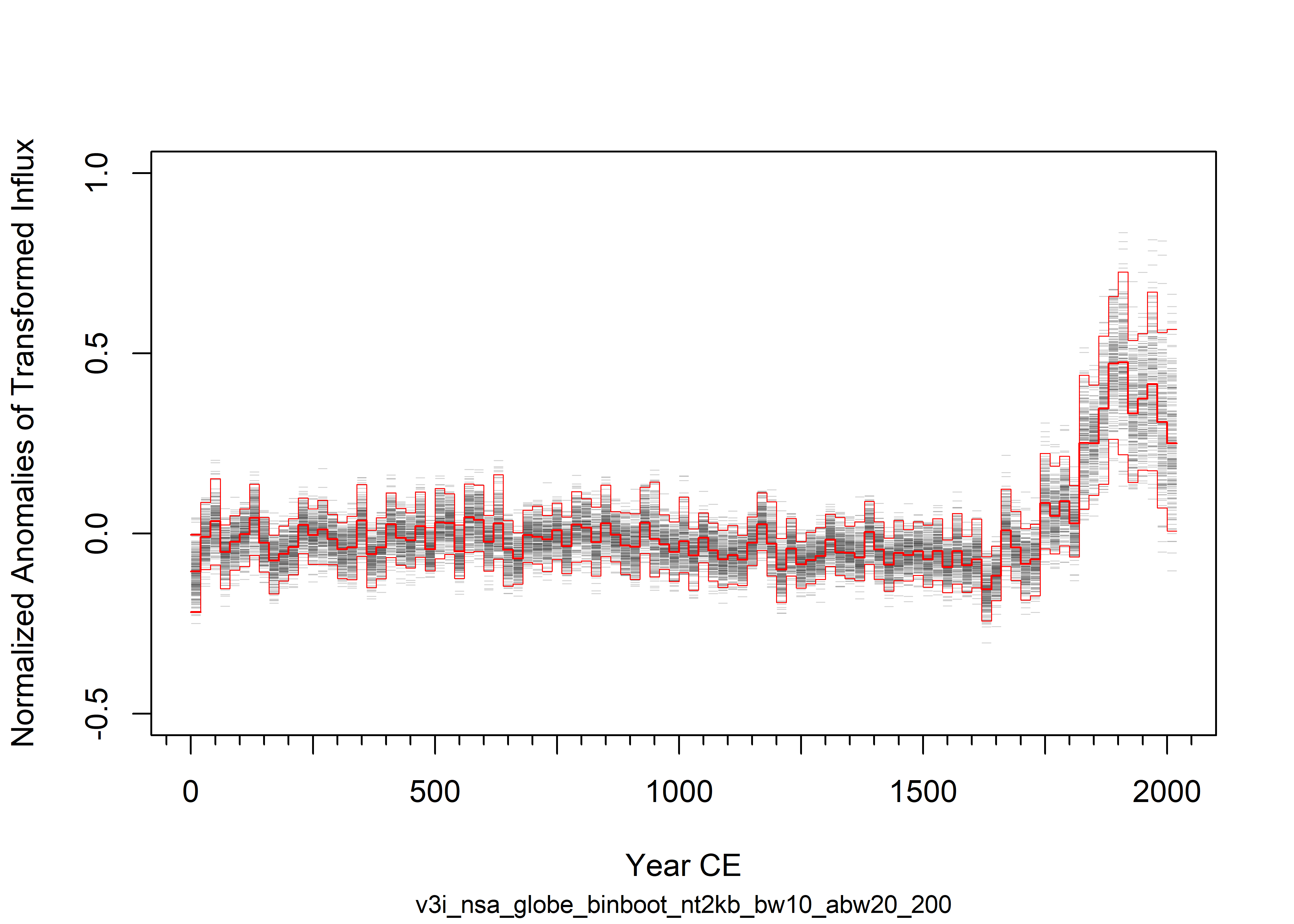

if (plotout == "pdf") {dev.off()}
if (plotout == "png") {dev.off()}
proc.time() - ptm

4.3 Output

The fitted curves are written out in the usual way.

curveout <- data.frame(cbind(abinage, 1950-abinage, bin_fit_all, yfit975, yfit025, ndec_tot, ninwin_tot))
colnames(curveout) <- c("age", "YearCE", "bin_ave", "cu95", "cl95", "nsites", "ninwin")
outputfile <- paste(curvecsvpath, curvefile, sep="")
write.table(curveout, outputfile, col.names=TRUE, row.names=FALSE, sep=",")

Composite curves and bootstrap C.I.’s via binning (bin-boot.R)